Global Sessions Pro NY/London/Tokyo - O/C/H/LGLOBAL SESSIONS PRO — NY / LONDON / TOKYO
Session Opens, Highs, Lows, Midpoints, Closes, Ranges & Killzones
OVERVIEW
Global Sessions Pro is a comprehensive session-mapping indicator designed for traders who rely on market structure, session context, and time-based behavior.
The indicator automatically plots New York, London, and Tokyo sessions, including:
• Session Open, High, Low, Midpoint, and Close
• Prior session levels projected forward
• Session range boxes
• Right-side labeled price levels (clearly identified)
• Stacked session summary labels (no overlap)
• Optional killzones and overlap windows
• Breakout alerts (prior or current session levels)
The script is fully timezone-aware, DST-safe, and works on any chart timeframe.
KEY FEATURES
SESSION MAPPING
For each session (NY / London / Tokyo), the indicator can display:
• Open
• High
• Low
• Midpoint (High + Low) / 2
• Close
Each level is drawn with its own horizontal line and optional right-side label, so there is never confusion about which line represents which level.
SESSION RANGE BOXES
Optional shaded boxes highlight the true session range as it develops in real time.
These are useful for visualizing:
• Compression vs expansion
• Relative session volatility
• Strength or weakness between sessions
Opacity and visibility are fully configurable.
RIGHT-SIDE LEVEL LABELS
Each session level can be labeled on the right edge of the chart, showing:
• Session name (NY / Lon / Tok)
• Level type (O / H / L / M / C)
• Optional price value
Examples:
NY H: 18234.25
Lon L: 18098.50
Tok M: 18142.75
This eliminates ambiguity when multiple session levels overlap or share similar colors.
SESSION SUMMARY LABELS (AUTO-STACKED)
At the top of each session range, an optional summary label displays:
• Session name
• Open / High / Low / Close
• Total range (points)
• Range in ticks
• ATR multiple
Summary labels are automatically stacked vertically using ATR-based or tick-based spacing, preventing overlap even when multiple sessions occur close together.
PRIOR SESSION LEVELS
The indicator can project prior session levels into the next session, including:
• Prior High and Low
• Optional prior Open, Close, and Midpoint
These levels are commonly used for:
• Support and resistance
• Liquidity sweeps
• Mean reversion
• Failed breakouts
Projection length is configurable and safely capped to comply with TradingView drawing limits.
KILLZONES AND SESSION OVERLAPS
Optional background shading highlights key institutional windows:
• London Open
• New York Open
• London / New York overlap
These zones help identify high-probability volatility windows and time-based trade filters.
All killzones respect the selected session timezone basis.
ALERTS
Built-in alerts are available for:
• Break of prior session high
• Break of prior session low
• Break of current session high
• Break of current session low
Alerts can be configured to trigger on wick or close.
Alert logic is written using precomputed crossover detection to ensure historical consistency and avoid missed or false alerts.
TIMEZONE AND SESSION HANDLING (IMPORTANT)
SESSION TIME BASIS OPTIONS
The indicator supports three session-time modes:
Market Local (DST-aware) – Recommended
• New York uses America/New_York
• London uses Europe/London
• Tokyo uses Asia/Tokyo
• Automatically adjusts for daylight saving time
UTC (Fixed)
• Sessions are interpreted strictly in UTC
• Best for crypto or non-DST workflows
• Requires manual adjustment during DST changes
Custom Timezone
• Define a single custom timezone for all sessions
This ensures sessions display correctly regardless of the chart’s timezone.
DEFAULT SESSION TIMES
(Default values assume Market Local (DST-aware) mode)
Tokyo: 09:00 – 15:00
London: 08:00 – 16:30
New York: 09:30 – 16:00
These defaults are optimized for cash and index trading.
FX traders may adjust session windows as needed.
BEST USE CASES
This indicator is particularly effective for:
• Index futures (ES, NQ, RTY, DAX, FTSE)
• Forex session-based strategies
• Time-based breakout systems
• Liquidity sweep and mean-reversion models
• London Open and New York Open trading
• Multi-session market context analysis
PERFORMANCE AND SAFETY NOTES
• All future-drawn objects are capped to comply with TradingView limits
• Crossover logic is evaluated every bar to prevent calculation drift
• Old session drawings are automatically culled to reduce chart clutter
• Works on all intraday and higher timeframes
RECOMMENDED SETTINGS
For most traders:
• Session Time Basis: Market Local (DST-aware)
• Show Open / High / Low / Midpoint: ON
• Prior Session Levels: ON
• Summary Labels: ON
• Killzones: ON
• Alerts: ON (Close-based)
FINAL NOTES
This indicator is designed to provide objective session structure without opinionated trade signals. It works best as a context layer combined with your own execution rules, confirmations, and risk management.
If you trade time, structure, and liquidity, this script provides the framework.
在脚本中搜索"session high"

Statistcal Daily Profile & Ranges# Statistical Daily Profile & Ranges - TradingView Publication Guide
## Overview
The **Statistical Daily Profile & Ranges** indicator is a comprehensive tool designed to analyze intraday session behavior and daily range characteristics. It combines Average Daily Range (ADR) projection levels with detailed session-by-session statistics and probability-based trading insights derived from historical price action patterns.
## What This Indicator Does
This indicator provides traders with three core analytical components:
1. **ADR Projection Levels** - Dynamic support/resistance levels based on historical daily ranges
2. **Session Range Analysis** - Visual boxes and statistical breakdowns for four key trading sessions
3. **Dynamic Probability Display** - Real-time probability statistics based on overnight session relationships
## How It Works
### Average Daily Range (ADR) Calculation
The indicator calculates the average daily range over a user-defined lookback period (default: 10 days) and projects this range from each day's opening price. This creates two key levels:
- **ADR High**: Opening price + average daily range
- **ADR Low**: Opening price - average daily range
- **ADR Median**: The opening price (middle of the projected range)
These levels are recalculated at the start of each trading day and extend forward, providing dynamic support and resistance zones based on recent volatility characteristics.
### Session Tracking & Statistics
The indicator monitors four distinct trading sessions (times in Eastern Time):
1. **Asia Session** (8:00 PM - 2:00 AM)
2. **London Session** (2:00 AM - 8:00 AM)
3. **NY Open** (8:00 AM - 9:00 AM)
4. **NY Initial Balance** (9:30 AM - 10:30 AM)
For each session, the indicator:
- Draws a colored box showing the session's high-to-low range
- Tracks the opening price, high, and low
- Stores historical data for statistical analysis
- Calculates average ranges by day of week (Monday through Friday)
The session statistics are displayed in a customizable table showing average point ranges for each session across different weekdays, helping traders identify which sessions and days typically produce the most movement.
### Dynamic Probability System
The indicator analyzes the relationship between the Asia and London sessions to determine the current market setup. After the London session closes, it automatically detects one of four possible conditions:
**1. London Engulfs Asia**
- London session breaks both above Asia's high AND below Asia's low
- This indicates strong momentum during the European session
- Most common occurrence pattern
**2. Asia Engulfs London**
- Asia session range completely contains the London session range
- Indicates consolidation during London hours
- Relatively rare pattern (occurs approximately 5.36% of the time)
**3. London Partially Engulfs Upwards**
- London breaks above Asia's high but stays above Asia's low
- Suggests bullish momentum continuation from Asia into London
**4. London Partially Engulfs Downwards**
- London breaks below Asia's low but stays below Asia's high
- Suggests bearish momentum continuation from Asia into London
Once a condition is detected, the indicator displays a probability table showing historically observed outcomes for that specific setup, including:
- Probability of NY session taking out key levels (Asia high/low, London high/low)
- Probability of NY session engulfing the entire overnight range
- Directional bias for NY Cash session (9:30 AM - 4:00 PM)
## How to Use This Indicator
### Initial Setup
1. Add the indicator to your chart (works on any intraday timeframe below Daily)
2. Adjust the **ADR Days** setting (default: 10) to control the lookback period for range calculation
3. Adjust the **Session Lookback Days** setting (default: 50) to determine how much historical data feeds the statistics tables
### Reading the ADR Levels
- Use the **ADR High** and **ADR Low** lines as potential profit targets or areas where price may encounter resistance
- The **ADR Median** line represents the opening price and can act as a pivot point for intraday directional bias
- If price reaches the ADR High early in the session, it suggests strong bullish momentum; conversely for ADR Low
- These levels adapt daily based on recent volatility, making them more responsive than static levels
### Interpreting Session Boxes
- **Session boxes** visually highlight when each trading session is active and its price range
- Larger boxes indicate higher volatility during that session
- Compare current session ranges to the statistical averages shown in the table
- Sessions that are unusually quiet or active relative to historical averages may signal compression or expansion
### Using the Session Statistics Table
- The table shows average point ranges for each session broken down by weekday
- Identify which sessions typically produce the most movement on specific days
- For example, if London on Thursdays averages 40 points while Mondays average 25 points, you can adjust position sizing or expectations accordingly
- The **Total** column shows the overall average across all days
- Sample sizes (shown in brackets if enabled) indicate data reliability
### Trading with the Probability Table
The probability table updates dynamically after the London session closes and shows statistically probable outcomes based on 12 years of NQ futures data.
**Important Limitations:**
- **These probabilities are derived from NQ (Nasdaq E-mini futures) data only**
- **Do NOT apply these probability statistics to other instruments** (ES, stocks, forex, etc.)
- The probabilities represent historical frequencies, not guarantees
- Always combine with your own analysis, risk management, and market context
**How to Apply the Probabilities:**
When **London Engulfs Asia**:
- Watch for NY session to take out London's extremes (72.33% probability for high, 71.12% for low)
- Slight bullish bias in NY Cash session (54.80% vs 45.20%)
- Lower probability of complete overnight engulfment (44.13%)
When **Asia Engulfs London** (rare - 5.36% occurrence):
- Higher probability NY takes Asia's high (75.86%)
- Moderately high probability NY takes Asia's low (65.52%)
- Slight increase in bullish bias (58.42% vs 41.58%)
- Recognize this as an unusual setup
When **London Partially Engulfs Upwards**:
- Very high probability NY takes London high (81.51%)
- Strong probability NY takes London low (64.45%)
- Moderate probability NY takes Asian low (53.16%)
- Slight bullish bias (55.52%)
When **London Partially Engulfs Downwards**:
- Very high probability NY takes London low (75.29%)
- Strong probability NY takes London high (68.80%)
- Moderate probability NY takes Asian high (56.44%)
- Slight bullish bias maintained (52.99%)
### Practical Trading Applications
**Scenario 1: Range Projection**
If the ADR is 500 points and the market opens at 25,000:
- ADR High: 25,500 (potential resistance/target)
- ADR Low: 24,500 (potential support/target)
- Monitor how price interacts with these levels throughout the day
**Scenario 2: Session-Based Trading**
Using the statistics table, you notice London on Wednesdays averages 35 points. During a Wednesday London session:
- If London has already moved 30 points, the session may be exhausting its typical range
- If London has only moved 15 points with an hour remaining, there may be expansion potential
- Adjust stop losses and targets based on typical session behavior
**Scenario 3: Probability-Based Setup**
It's 8:05 AM ET and the indicator shows "London Partially Engulfs Upwards":
- You now know there's an 81.51% historical probability NY will take out London's high
- There's a 53.16% probability NY will reach down to Asia's low
- The NY Cash session has a slight bullish bias (55.52%)
- Consider this alongside your technical analysis for directional bias and level targeting
## Customization Options
### Visual Settings
- **Line Width**: Adjust thickness of ADR levels
- **ADR Color/Style**: Customize appearance of ADR projection lines (solid, dashed, dotted)
- **Median Line**: Toggle visibility and customize appearance separately
- **Session Box Colors**: Customize each session's box color independently
- **Show Session Boxes**: Toggle session box visibility on/off
### Label Settings
- **ADR Labels**: Show/hide labels for ADR High and ADR Low, adjust size
- **Median Label**: Separate control for median line label
- **Session Labels**: Show/hide session name labels, adjust size
- **Label Colors**: Customize text colors for all labels
### Table Settings
- **Session Stats Table**: Position (9 locations available), size (Tiny to Huge), toggle on/off
- **Sample Sizes**: Show/hide the number of historical samples used for each calculation
- **Probabilities Table**: Separate position and size controls, toggle on/off
### Session Times
- Each session's time range can be customized to fit different markets or preferences
- All times are in Eastern Time (America/New_York timezone)
## Technical Notes
### Data Requirements
- The indicator requires sufficient historical data based on your lookback settings
- Minimum recommended: 50+ days of intraday data for reliable statistics
- Works on any timeframe below Daily (1-minute, 5-minute, 15-minute, etc.)
### Calculation Methodology
- **ADR Calculation**: Simple average of absolute daily high-low ranges
- **Session Statistics**: Mean average of ranges for each session filtered by day of week
- **Condition Detection**: Boolean logic comparing session high/low relationships
- All calculations update in real-time as new bars form
### Probability Data Source
The probability statistics displayed in the dynamic table are derived from:
- **Dataset**: 12 years of NQ (Nasdaq E-mini futures) historical data
- **Methodology**: Frequency analysis of outcomes following specific setup conditions
- **Time Period**: Multiple market cycles including various volatility regimes
**Critical Warning**: These probabilities are specific to NQ and reflect that instrument's behavior patterns. Market microstructure, participant behavior, and volatility characteristics differ significantly across instruments. Do not apply these NQ-derived probabilities to other markets (ES, RTY, YM, individual stocks, forex, commodities, etc.).
## Best Practices
1. **Combine with Other Analysis**: Use this indicator as one component of a complete trading methodology, not a standalone system
2. **Respect Risk Management**: Probabilities are not certainties; always use proper position sizing and stop losses
3. **Context Matters**: High-impact news events, holiday trading, and extreme volatility can invalidate typical patterns
4. **Verify Statistics**: Monitor your own results and compare to the displayed probabilities
5. **Adapt Session Times**: If trading instruments with different active hours, adjust session times accordingly
6. **Regular Calibration**: Periodically review if the session averages and probabilities remain relevant to current market conditions
## Understanding Originality
This indicator is original in its approach to combining three analytical frameworks into a single tool:
1. **Dynamic ADR Projection**: Unlike static pivot points, these levels adapt daily based on recent volatility
2. **Session-Specific Statistics**: Goes beyond simple volume profiles by quantifying average ranges for specific time windows across weekdays
3. **Conditional Probability Display**: Automatically detects overnight session relationships and displays relevant probability data rather than showing all scenarios simultaneously
The conditional logic system that determines which probability set to display is a key differentiator—traders only see the statistics relevant to the current market setup, reducing information overload and improving decision-making clarity.
## Summary
The **Statistical Daily Profile & Ranges** indicator provides traders with a comprehensive framework for understanding daily range potential, session-specific behavior patterns, and probability-based setup analysis. By combining ADR projection levels with detailed session statistics and dynamic probability displays, traders gain multiple perspectives on potential price movement within the trading day.
The indicator is most effective when used to:
- Set realistic profit targets based on average daily range
- Identify which sessions typically produce movement on specific weekdays
- Understand probability-weighted outcomes for different overnight setup conditions (NQ only)
- Visualize session ranges and compare them to historical averages
Remember that all statistical analysis reflects historical patterns, and market behavior can change. Always combine indicator signals with sound risk management, proper position sizing, and your own market analysis.

Session Sweep System – WarRoomXYZ V1WarRoom Session Sweep System v1 is a open-source institutional trading framework built to identify liquidity behavior across Asia, London, and New York sessions.
It combines session-based liquidity mapping, sweep detection, daily expansion modeling, and trend confirmation into a unified, timing-driven system optimized for XAUUSD, FX pairs, indices, and any instrument with session-dependent volatility.
This tool does not attempt to predict direction with arbitrary oscillators.
Instead, it focuses on the underlying market mechanisms that drive price:
liquidity, timing, expansion, and trend alignment.
Below is a detailed explanation of what the script does, how its components work, and how traders can use it effectively.
🔹 1. Session Liquidity Mapping
The script automatically identifies the Asia (00:00–06:00 GMT), London (07:00–12:00 GMT), and New York (13:00–17:00 GMT) sessions and builds real-time session ranges.
Each session creates a liquidity pool.
Trading institutions frequently sweep the high or low of one session before delivering the real move in the next session.
This script captures that behavior by:
►Drawing session range boxes
►Tracking previous session highs/lows
►Highlighting high-probability sweep locations
These ranges are essential reference points for timing entries and exits.
🔹 2. Liquidity Sweep Detection (Buy & Sell Sweeps)
The indicator identifies when price runs a previous session high/low and rejects back inside the range, which is commonly interpreted as a liquidity sweep.
The following sweep types are monitored:
►London sweeping Asia
►New York sweeping London
►Asia sweeping New York
►Daily sweep of PDH/PDL
Sweeps signal that liquidity has been collected and that a potential reversal or continuation is likely.
These are marked clearly on the chart for real-time decision-making.
🔹 3. Killzone Timing Model (GMT Time)
Market manipulation and expansion often occur during specific time windows.
The script highlights these institutional killzones:
►London Killzone: 07:00–10:00 GMT
►New York Killzone: 13:30–15:30 GMT
►NY PM Session: 19:00–21:00 GMT
Sweeps occurring inside these windows carry a significantly higher probability.
The timing layer helps filter out low-quality setups.
🔹 4. Daily Range & ADR Expansion Engine
A dedicated panel displays:
►Current day range
►ADR (Average Daily Range)
►Expansion stage (Early / Developed / Extended)
►PDH/PDL swept or intact
►Overall session bias
This allows traders to understand whether the daily move is likely to continue or reverse.
For example:
►Early expansion → trend continuation likely
►Extended expansion → reversal setups become more probable
This is useful for intraday targets and risk management.
🔹 5. MA Cloud Trend Model (Fast/Slow Structure)
To align liquidity behavior with directional conviction, the script includes a configurable MA engine:
►Fast & slow MA
►MA cloud
►Slope-based trend coloring
►Trend background
►MA cross alerts
The cloud provides trend confirmation without relying on oscillators.
Trades are higher quality when the sweep direction aligns with the MA trend.
🔹 6. How the Components Work Together
The script integrates several institutional concepts into one coherent model:
►Sessions define liquidity pools
►Sweeps identify stop-hunts and reversals
►Killzones define optimal timing
►MA Cloud confirms directional bias
►ADR engine indicates expansion potential
This creates a structured framework:
Sweep → Timing → Trend → Expansion → Execution
Each component strengthens the others, forming a robust decision-making model.
🔹 7. How to Use the Indicator (Practical Guide)
✔ Look for a sweep of a previous session level
When price runs a session high/low and closes back inside, liquidity has likely been collected.
✔ Confirm timing
Sweeps inside London or NY killzones tend to produce the strongest moves.
✔ Confirm trend
Use MA cloud direction and slope:
►Cloud green → long setups preferred
►Cloud red → short setups preferred
✔ Check ADR panel
If the day has already expanded significantly, reversal setups are more likely.
If expansion is still early, continuation setups are favored.
✔ Plan your trade
Common targets include:
►Opposite side of session range
►ADR High/Low
►PDH/PDL
Stops are typically placed beyond the sweep wick.
This creates a repeatable, rule-based approach to intraday liquidity trading.
🔹 8. Why This Script Is Original
This is not a mashup of existing open-source indicators.
It introduces:
►A custom session-linked liquidity sweep engine
►A structured daily expansion model
►Integrated killzone timing aligned with GMT
►A unified bias panel merging sweeps, ADR, and session manipulation
►A trend confirmation layer designed around session behavior
While it uses known institutional concepts, their integration, execution, and timing framework are unique, purpose-built, and not directly found in open-source scripts.
🔹 9. Suitable Markets
This indicator works best on:
►XAUUSD
►Major FX pairs
►US indices
►Synthetic markets with session cycles
Ideal timeframes: 1m, 5m, 15m, 30m
🔹 10. Limitations / Notes
This is an analytical tool, not a buy/sell signal generator
All sweeps are confirmed at candle close (non-repaint)
The tool assumes GMT session windows unless chart time differs
Users must practice risk management and entry triggers manually
Disclaimer
This script is provided for informational and educational purposes only. It does not provide financial, investment, or trading advice, and it does not guarantee profits or future performance. All decisions made based on this script are solely the responsibility of the user.
This script does not execute trades, manage risk, or replace the need for trader discretion. Market behavior can change quickly, and past behavior detected by the script does not ensure similar future outcomes.
Users should test the script on demo or simulation environments before applying it to live markets and must maintain full responsibility for their own risk management, position sizing, and trade execution.
Trading involves risk, and losses can exceed deposits. By using this script, you acknowledge that you understand and accept all associated risks.

FX OSINT - Institutional Midnight Intelligence For ForexFX OSINT — Institutional Midnight Intelligence For Forex
See Your FX Charts Like an Intelligence Briefing, Not a Guess
If you’ve ever stared at EURUSD or GBPJPY and thought:
Where is the real liquidity?
Is this move sponsored by smart money or just noise?
Am I buying into premium or discount?
…then FX OSINT is designed for you.
FX OSINT (Forex Open Source Intelligence) treats the FX market the way an analyst treats an investigation:
Collect open‑source signals from price, time, and volatility.
Map out liquidity, structure, and sessions in a repeatable way.
Present them in a clean, non‑cluttered dashboard so you can read context quickly.
No rainbow spaghetti. No 12 indicators stacked on top of each other. Just structured information, midnight visuals, and a clear read on what the market is doing right now.
Why FX OSINT Exists
Many FX traders run into the same problems:
Overloaded charts – multiple indicators fighting for space, none talking to each other.
Signals with no context – arrows that ignore structure, sessions, and liquidity.
Tools not tuned for FX – generic indicators that don’t care what pair you are on.
FX OSINT brings this together into one FX‑focused framework that:
Understands structure : BOS/CHOCH, swings, and trend across multiple timeframes.
Respects liquidity : sweeps, order blocks, and FVGs with controlled visibility.
Reads volatility & ADR : how far today’s range has developed.
Knows the clock : London, New York, and key killzones.
Scores confluence : a 0–100 engine that summarizes how much is lining up.
FX OSINT is built for traders who want structured, institutional‑style logic with a disciplined, midnight‑themed UI —not flashing buy/sell buttons.
1. Midnight Dashboard — Top‑Right Intelligence Panel
This panel acts as your compact “situation room”:
CONFLUENCE — 0–100 score blending trend alignment, volatility regime, sessions, liquidity events, order blocks, FVGs, and ADR context.
REGIME — Low / Building / Normal / Expansion / Extreme, driven by ATR relationships, so you know if you’re in chop, trend, or expansion.
HTF / MTF / LTF TREND — Higher‑, medium‑, and current‑timeframe bias in one place, so you see if you are trading with or against the larger flow.
ADR USED — How much of today’s typical range has already been consumed in percentage terms.
PIP VALUE — Approximate pip size per pair, including JPY‑style pairs.
Everything is bold, legible, and color‑coded, but the layout stays minimal so you can:
Look once → understand the context.
2. Structure, BOS, CHOCH — Smart‑Money‑Style Skeleton
FX OSINT tracks swing highs and lows, then shows how structure evolves:
Trend logic based on evolving swings, not just a moving average cross.
BOS (Break of Structure) when price expands in the direction of trend.
CHOCH (Change of Character) when behavior flips and the market structure changes.
Labels are selective, not spammy . You don’t get a tag on every minor wiggle—only when structure meaningfully shifts, so it’s easier to answer:
"Are we continuing the current leg, or did something actually change here?"
3. Liquidity Sweeps, Order Blocks & FVGs — The OSINT Layer
FX OSINT treats liquidity as a key information layer:
Liquidity sweeps — Detects when price spikes through recent highs/lows and then snaps back, flagging potential stop runs.
Order blocks — The last opposite candle before a displacement move, drawn as controlled boxes with limited lifespan to avoid clutter.
Fair Value Gaps (FVGs) — Three‑candle imbalances rendered as precise zones with a cap on how many can exist at once.
Under the hood, boxes are managed so your chart does not become a wall of old zones:
// Draw Order Blocks with overlap prevention
if isBullishOB and showOrderBlocks
if array.size(obBoxes) >= maxBoxes
oldBox = array.shift(obBoxes)
box.delete(oldBox)
newBox = box.new(bar_index , low , bar_index + obvLength, high ,
border_color = bullColor, bgcolor = bullColorTransp,
border_width = 2, extend = extend.none)
array.push(obBoxes, newBox)
Box limits keep the number of zones under control.
Borders and transparency are tuned so you still see price clearly.
You end up with a curated liquidity map , rather than a chart buried under every level price has ever touched.
4. Volatility, ADR & Sessions — Time and Range Intelligence
FX OSINT runs a Volatility Regime Analyzer and an ADR engine in the background:
Volatility regime — Five states (Low → Extreme) derived from fast vs. slow ATR.
ADR bands — Daily high/mid/low projected from the current daily open.
ADR used % — How far today’s move has traveled relative to its typical range.
On the time side:
Asia, London, New York sessions are softly highlighted with a single active background to avoid overlapping colors.
Killzones (e.g., London and New York opens) can be emphasized when you want to focus on where significant moves often begin.
Together, this helps you answer:
"What time is it in the trading day?"
"How stretched are we?"
"Is expansion just starting, or are we late to the move?"
5. ICT‑Style Add‑Ons — BOS/CHOCH, Premium/Discount, and Confluence
For modern FX / ICT‑inspired workflows, FX OSINT includes:
BOS / CHOCH labels — Clear structural shifts based on swings.
Premium / Discount zones — 25%, 50%, 75% levels of the daily range, so you know if you are buying discount in an uptrend or selling premium in a downtrend.
Confluence score — A single number summarizing how many conditions line up in the current context.
Instead of replacing your plan, FX OSINT compresses your checklist into the chart:
Structure
Liquidity
Session / Time
Volatility / ADR
Higher‑timeframe alignment
When these agree, the dashboard reflects it. When they don’t, it stays neutral and lets you see the conflict.
How To Use FX OSINT
FX OSINT is not a signal bot. It is an information engine that organizes context so you can apply your own plan.
A typical workflow might look like:
Start on higher timeframes (e.g., H4/D1) to form directional bias from structure, volatility regime, and ADR context.
Move to intraday timeframes (e.g., M15/H1) around your chosen sessions (London and/or New York).
Look for confluence :
HTF / MTF / LTF trends aligned.
Price in discount for longs or premium for shorts.
Recent liquidity sweep into a meaningful OB or FVG.
Confluence score at or above a level you consider significant.
Then refine entries using BOS/CHOCH on lower timeframes according to your own risk and execution rules.
FX OSINT aims to make sure you do not enter a trade without seeing:
Where you are in the day (ADR and sessions).
Where you are in the volatility cycle (regime).
Who currently appears in control (structure and trend).
Which liquidity was just targeted (sweeps and zones).
Design Choices and Scope
FX OSINT was designed around a few clear constraints:
FX‑focused — Logic and filters tuned for FX majors, minors, exotics, and metals. It is intended for FX markets, not for every possible asset class.
Open‑source — The full Pine Script code is available so you can read it, learn from it, and adapt it to your own workflow if needed.
Clear themes — Two main visual styles (e.g., dark institutional “midnight” and a lighter accent variant) with a focus on readability, not visual noise.
Chart‑friendly — Panels use fixed areas, session highlights avoid overlapping, and boxes are capped/pruned so the chart remains usable.
FX OSINT is for only Forex pairs, not anything else!
Hope you enjoyed and remember your Open Source Intelligence Matters 😉!
-officialjackofalltrades

Dimensional Resonance ProtocolDimensional Resonance Protocol
🌀 CORE INNOVATION: PHASE SPACE RECONSTRUCTION & EMERGENCE DETECTION
The Dimensional Resonance Protocol represents a paradigm shift from traditional technical analysis to complexity science. Rather than measuring price levels or indicator crossovers, DRP reconstructs the hidden attractor governing market dynamics using Takens' embedding theorem, then detects emergence —the rare moments when multiple dimensions of market behavior spontaneously synchronize into coherent, predictable states.
The Complexity Hypothesis:
Markets are not simple oscillators or random walks—they are complex adaptive systems existing in high-dimensional phase space. Traditional indicators see only shadows (one-dimensional projections) of this higher-dimensional reality. DRP reconstructs the full phase space using time-delay embedding, revealing the true structure of market dynamics.
Takens' Embedding Theorem (1981):
A profound mathematical result from dynamical systems theory: Given a time series from a complex system, we can reconstruct its full phase space by creating delayed copies of the observation.
Mathematical Foundation:
From single observable x(t), create embedding vectors:
X(t) =
Where:
• d = Embedding dimension (default 5)
• τ = Time delay (default 3 bars)
• x(t) = Price or return at time t
Key Insight: If d ≥ 2D+1 (where D is the true attractor dimension), this embedding is topologically equivalent to the actual system dynamics. We've reconstructed the hidden attractor from a single price series.
Why This Matters:
Markets appear random in one dimension (price chart). But in reconstructed phase space, structure emerges—attractors, limit cycles, strange attractors. When we identify these structures, we can detect:
• Stable regions : Predictable behavior (trade opportunities)
• Chaotic regions : Unpredictable behavior (avoid trading)
• Critical transitions : Phase changes between regimes
Phase Space Magnitude Calculation:
phase_magnitude = sqrt(Σ ² for i = 0 to d-1)
This measures the "energy" or "momentum" of the market trajectory through phase space. High magnitude = strong directional move. Low magnitude = consolidation.
📊 RECURRENCE QUANTIFICATION ANALYSIS (RQA)
Once phase space is reconstructed, we analyze its recurrence structure —when does the system return near previous states?
Recurrence Plot Foundation:
A recurrence occurs when two phase space points are closer than threshold ε:
R(i,j) = 1 if ||X(i) - X(j)|| < ε, else 0
This creates a binary matrix showing when the system revisits similar states.
Key RQA Metrics:
1. Recurrence Rate (RR):
RR = (Number of recurrent points) / (Total possible pairs)
• RR near 0: System never repeats (highly stochastic)
• RR = 0.1-0.3: Moderate recurrence (tradeable patterns)
• RR > 0.5: System stuck in attractor (ranging market)
• RR near 1: System frozen (no dynamics)
Interpretation: Moderate recurrence is optimal —patterns exist but market isn't stuck.
2. Determinism (DET):
Measures what fraction of recurrences form diagonal structures in the recurrence plot. Diagonals indicate deterministic evolution (trajectory follows predictable paths).
DET = (Recurrence points on diagonals) / (Total recurrence points)
• DET < 0.3: Random dynamics
• DET = 0.3-0.7: Moderate determinism (patterns with noise)
• DET > 0.7: Strong determinism (technical patterns reliable)
Trading Implication: Signals are prioritized when DET > 0.3 (deterministic state) and RR is moderate (not stuck).
Threshold Selection (ε):
Default ε = 0.10 × std_dev means two states are "recurrent" if within 10% of a standard deviation. This is tight enough to require genuine similarity but loose enough to find patterns.
🔬 PERMUTATION ENTROPY: COMPLEXITY MEASUREMENT
Permutation entropy measures the complexity of a time series by analyzing the distribution of ordinal patterns.
Algorithm (Bandt & Pompe, 2002):
1. Take overlapping windows of length n (default n=4)
2. For each window, record the rank order pattern
Example: → pattern (ranks from lowest to highest)
3. Count frequency of each possible pattern
4. Calculate Shannon entropy of pattern distribution
Mathematical Formula:
H_perm = -Σ p(π) · ln(p(π))
Where π ranges over all n! possible permutations, p(π) is the probability of pattern π.
Normalized to :
H_norm = H_perm / ln(n!)
Interpretation:
• H < 0.3 : Very ordered, crystalline structure (strong trending)
• H = 0.3-0.5 : Ordered regime (tradeable with patterns)
• H = 0.5-0.7 : Moderate complexity (mixed conditions)
• H = 0.7-0.85 : Complex dynamics (challenging to trade)
• H > 0.85 : Maximum entropy (nearly random, avoid)
Entropy Regime Classification:
DRP classifies markets into five entropy regimes:
• CRYSTALLINE (H < 0.3): Maximum order, persistent trends
• ORDERED (H < 0.5): Clear patterns, momentum strategies work
• MODERATE (H < 0.7): Mixed dynamics, adaptive required
• COMPLEX (H < 0.85): High entropy, mean reversion better
• CHAOTIC (H ≥ 0.85): Near-random, minimize trading
Why Permutation Entropy?
Unlike traditional entropy methods requiring binning continuous data (losing information), permutation entropy:
• Works directly on time series
• Robust to monotonic transformations
• Computationally efficient
• Captures temporal structure, not just distribution
• Immune to outliers (uses ranks, not values)
⚡ LYAPUNOV EXPONENT: CHAOS vs STABILITY
The Lyapunov exponent λ measures sensitivity to initial conditions —the hallmark of chaos.
Physical Meaning:
Two trajectories starting infinitely close will diverge at exponential rate e^(λt):
Distance(t) ≈ Distance(0) × e^(λt)
Interpretation:
• λ > 0 : Positive Lyapunov exponent = CHAOS
- Small errors grow exponentially
- Long-term prediction impossible
- System is sensitive, unpredictable
- AVOID TRADING
• λ ≈ 0 : Near-zero = CRITICAL STATE
- Edge of chaos
- Transition zone between order and disorder
- Moderate predictability
- PROCEED WITH CAUTION
• λ < 0 : Negative Lyapunov exponent = STABLE
- Small errors decay
- Trajectories converge
- System is predictable
- OPTIMAL FOR TRADING
Estimation Method:
DRP estimates λ by tracking how quickly nearby states diverge over a rolling window (default 20 bars):
For each bar i in window:
δ₀ = |x - x | (initial separation)
δ₁ = |x - x | (previous separation)
if δ₁ > 0:
ratio = δ₀ / δ₁
log_ratios += ln(ratio)
λ ≈ average(log_ratios)
Stability Classification:
• STABLE : λ < 0 (negative growth rate)
• CRITICAL : |λ| < 0.1 (near neutral)
• CHAOTIC : λ > 0.2 (strong positive growth)
Signal Filtering:
By default, NEXUS requires λ < 0 (stable regime) for signal confirmation. This filters out trades during chaotic periods when technical patterns break down.
📐 HIGUCHI FRACTAL DIMENSION
Fractal dimension measures self-similarity and complexity of the price trajectory.
Theoretical Background:
A curve's fractal dimension D ranges from 1 (smooth line) to 2 (space-filling curve):
• D ≈ 1.0 : Smooth, persistent trending
• D ≈ 1.5 : Random walk (Brownian motion)
• D ≈ 2.0 : Highly irregular, space-filling
Higuchi Method (1988):
For a time series of length N, construct k different curves by taking every k-th point:
L(k) = (1/k) × Σ|x - x | × (N-1)/(⌊(N-m)/k⌋ × k)
For different values of k (1 to k_max), calculate L(k). The fractal dimension is the slope of log(L(k)) vs log(1/k):
D = slope of log(L) vs log(1/k)
Market Interpretation:
• D < 1.35 : Strong trending, persistent (Hurst > 0.5)
- TRENDING regime
- Momentum strategies favored
- Breakouts likely to continue
• D = 1.35-1.45 : Moderate persistence
- PERSISTENT regime
- Trend-following with caution
- Patterns have meaning
• D = 1.45-1.55 : Random walk territory
- RANDOM regime
- Efficiency hypothesis holds
- Technical analysis least reliable
• D = 1.55-1.65 : Anti-persistent (mean-reverting)
- ANTI-PERSISTENT regime
- Oscillator strategies work
- Overbought/oversold meaningful
• D > 1.65 : Highly complex, choppy
- COMPLEX regime
- Avoid directional bets
- Wait for regime change
Signal Filtering:
Resonance signals (secondary signal type) require D < 1.5, indicating trending or persistent dynamics where momentum has meaning.
🔗 TRANSFER ENTROPY: CAUSAL INFORMATION FLOW
Transfer entropy measures directed causal influence between time series—not just correlation, but actual information transfer.
Schreiber's Definition (2000):
Transfer entropy from X to Y measures how much knowing X's past reduces uncertainty about Y's future:
TE(X→Y) = H(Y_future | Y_past) - H(Y_future | Y_past, X_past)
Where H is Shannon entropy.
Key Properties:
1. Directional : TE(X→Y) ≠ TE(Y→X) in general
2. Non-linear : Detects complex causal relationships
3. Model-free : No assumptions about functional form
4. Lag-independent : Captures delayed causal effects
Three Causal Flows Measured:
1. Volume → Price (TE_V→P):
Measures how much volume patterns predict price changes.
• TE > 0 : Volume provides predictive information about price
- Institutional participation driving moves
- Volume confirms direction
- High reliability
• TE ≈ 0 : No causal flow (weak volume/price relationship)
- Volume uninformative
- Caution on signals
• TE < 0 (rare): Suggests price leading volume
- Potentially manipulated or thin market
2. Volatility → Momentum (TE_σ→M):
Does volatility expansion predict momentum changes?
• Positive TE : Volatility precedes momentum shifts
- Breakout dynamics
- Regime transitions
3. Structure → Price (TE_S→P):
Do support/resistance patterns causally influence price?
• Positive TE : Structural levels have causal impact
- Technical levels matter
- Market respects structure
Net Causal Flow:
Net_Flow = TE_V→P + 0.5·TE_σ→M + TE_S→P
• Net > +0.1 : Bullish causal structure
• Net < -0.1 : Bearish causal structure
• |Net| < 0.1 : Neutral/unclear causation
Causal Gate:
For signal confirmation, NEXUS requires:
• Buy signals : TE_V→P > 0 AND Net_Flow > 0.05
• Sell signals : TE_V→P > 0 AND Net_Flow < -0.05
This ensures volume is actually driving price (causal support exists), not just correlated noise.
Implementation Note:
Computing true transfer entropy requires discretizing continuous data into bins (default 6 bins) and estimating joint probability distributions. NEXUS uses a hybrid approach combining TE theory with autocorrelation structure and lagged cross-correlation to approximate information transfer in computationally efficient manner.
🌊 HILBERT PHASE COHERENCE
Phase coherence measures synchronization across market dimensions using Hilbert transform analysis.
Hilbert Transform Theory:
For a signal x(t), the Hilbert transform H (t) creates an analytic signal:
z(t) = x(t) + i·H (t) = A(t)·e^(iφ(t))
Where:
• A(t) = Instantaneous amplitude
• φ(t) = Instantaneous phase
Instantaneous Phase:
φ(t) = arctan(H (t) / x(t))
The phase represents where the signal is in its natural cycle—analogous to position on a unit circle.
Four Dimensions Analyzed:
1. Momentum Phase : Phase of price rate-of-change
2. Volume Phase : Phase of volume intensity
3. Volatility Phase : Phase of ATR cycles
4. Structure Phase : Phase of position within range
Phase Locking Value (PLV):
For two signals with phases φ₁(t) and φ₂(t), PLV measures phase synchronization:
PLV = |⟨e^(i(φ₁(t) - φ₂(t)))⟩|
Where ⟨·⟩ is time average over window.
Interpretation:
• PLV = 0 : Completely random phase relationship (no synchronization)
• PLV = 0.5 : Moderate phase locking
• PLV = 1 : Perfect synchronization (phases locked)
Pairwise PLV Calculations:
• PLV_momentum-volume : Are momentum and volume cycles synchronized?
• PLV_momentum-structure : Are momentum cycles aligned with structure?
• PLV_volume-structure : Are volume and structural patterns in phase?
Overall Phase Coherence:
Coherence = (PLV_mom-vol + PLV_mom-struct + PLV_vol-struct) / 3
Signal Confirmation:
Emergence signals require coherence ≥ threshold (default 0.70):
• Below 0.70: Dimensions not synchronized, no coherent market state
• Above 0.70: Dimensions in phase, coherent behavior emerging
Coherence Direction:
The summed phase angles indicate whether synchronized dimensions point bullish or bearish:
Direction = sin(φ_momentum) + 0.5·sin(φ_volume) + 0.5·sin(φ_structure)
• Direction > 0 : Phases pointing upward (bullish synchronization)
• Direction < 0 : Phases pointing downward (bearish synchronization)
🌀 EMERGENCE SCORE: MULTI-DIMENSIONAL ALIGNMENT
The emergence score aggregates all complexity metrics into a single 0-1 value representing market coherence.
Eight Components with Weights:
1. Phase Coherence (20%):
Direct contribution: coherence × 0.20
Measures dimensional synchronization.
2. Entropy Regime (15%):
Contribution: (0.6 - H_perm) / 0.6 × 0.15 if H < 0.6, else 0
Rewards low entropy (ordered, predictable states).
3. Lyapunov Stability (12%):
• λ < 0 (stable): +0.12
• |λ| < 0.1 (critical): +0.08
• λ > 0.2 (chaotic): +0.0
Requires stable, predictable dynamics.
4. Fractal Dimension Trending (12%):
Contribution: (1.45 - D) / 0.45 × 0.12 if D < 1.45, else 0
Rewards trending fractal structure (D < 1.45).
5. Dimensional Resonance (12%):
Contribution: |dimensional_resonance| × 0.12
Measures alignment across momentum, volume, structure, volatility dimensions.
6. Causal Flow Strength (9%):
Contribution: |net_causal_flow| × 0.09
Rewards strong causal relationships.
7. Phase Space Embedding (10%):
Contribution: min(|phase_magnitude_norm|, 3.0) / 3.0 × 0.10 if |magnitude| > 1.0
Rewards strong trajectory in reconstructed phase space.
8. Recurrence Quality (10%):
Contribution: determinism × 0.10 if DET > 0.3 AND 0.1 < RR < 0.8
Rewards deterministic patterns with moderate recurrence.
Total Emergence Score:
E = Σ(components) ∈
Capped at 1.0 maximum.
Emergence Direction:
Separate calculation determining bullish vs bearish:
• Dimensional resonance sign
• Net causal flow sign
• Phase magnitude correlation with momentum
Signal Threshold:
Default emergence_threshold = 0.75 means 75% of maximum possible emergence score required to trigger signals.
Why Emergence Matters:
Traditional indicators measure single dimensions. Emergence detects self-organization —when multiple independent dimensions spontaneously align. This is the market equivalent of a phase transition in physics, where microscopic chaos gives way to macroscopic order.
These are the highest-probability trade opportunities because the entire system is resonating in the same direction.
🎯 SIGNAL GENERATION: EMERGENCE vs RESONANCE
DRP generates two tiers of signals with different requirements:
TIER 1: EMERGENCE SIGNALS (Primary)
Requirements:
1. Emergence score ≥ threshold (default 0.75)
2. Phase coherence ≥ threshold (default 0.70)
3. Emergence direction > 0.2 (bullish) or < -0.2 (bearish)
4. Causal gate passed (if enabled): TE_V→P > 0 and net_flow confirms direction
5. Stability zone (if enabled): λ < 0 or |λ| < 0.1
6. Price confirmation: Close > open (bulls) or close < open (bears)
7. Cooldown satisfied: bars_since_signal ≥ cooldown_period
EMERGENCE BUY:
• All above conditions met with bullish direction
• Market has achieved coherent bullish state
• Multiple dimensions synchronized upward
EMERGENCE SELL:
• All above conditions met with bearish direction
• Market has achieved coherent bearish state
• Multiple dimensions synchronized downward
Premium Emergence:
When signal_quality (emergence_score × phase_coherence) > 0.7:
• Displayed as ★ star symbol
• Highest conviction trades
• Maximum dimensional alignment
Standard Emergence:
When signal_quality 0.5-0.7:
• Displayed as ◆ diamond symbol
• Strong signals but not perfect alignment
TIER 2: RESONANCE SIGNALS (Secondary)
Requirements:
1. Dimensional resonance > +0.6 (bullish) or < -0.6 (bearish)
2. Fractal dimension < 1.5 (trending/persistent regime)
3. Price confirmation matches direction
4. NOT in chaotic regime (λ < 0.2)
5. Cooldown satisfied
6. NO emergence signal firing (resonance is fallback)
RESONANCE BUY:
• Dimensional alignment without full emergence
• Trending fractal structure
• Moderate conviction
RESONANCE SELL:
• Dimensional alignment without full emergence
• Bearish resonance with trending structure
• Moderate conviction
Displayed as small ▲/▼ triangles with transparency.
Signal Hierarchy:
IF emergence conditions met:
Fire EMERGENCE signal (★ or ◆)
ELSE IF resonance conditions met:
Fire RESONANCE signal (▲ or ▼)
ELSE:
No signal
Cooldown System:
After any signal fires, cooldown_period (default 5 bars) must elapse before next signal. This prevents signal clustering during persistent conditions.
Cooldown tracks using bar_index:
bars_since_signal = current_bar_index - last_signal_bar_index
cooldown_ok = bars_since_signal >= cooldown_period
🎨 VISUAL SYSTEM: MULTI-LAYER COMPLEXITY
DRP provides rich visual feedback across four distinct layers:
LAYER 1: COHERENCE FIELD (Background)
Colored background intensity based on phase coherence:
• No background : Coherence < 0.5 (incoherent state)
• Faint glow : Coherence 0.5-0.7 (building coherence)
• Stronger glow : Coherence > 0.7 (coherent state)
Color:
• Cyan/teal: Bullish coherence (direction > 0)
• Red/magenta: Bearish coherence (direction < 0)
• Blue: Neutral coherence (direction ≈ 0)
Transparency: 98 minus (coherence_intensity × 10), so higher coherence = more visible.
LAYER 2: STABILITY/CHAOS ZONES
Background color indicating Lyapunov regime:
• Green tint (95% transparent): λ < 0, STABLE zone
- Safe to trade
- Patterns meaningful
• Gold tint (90% transparent): |λ| < 0.1, CRITICAL zone
- Edge of chaos
- Moderate risk
• Red tint (85% transparent): λ > 0.2, CHAOTIC zone
- Avoid trading
- Unpredictable behavior
LAYER 3: DIMENSIONAL RIBBONS
Three EMAs representing dimensional structure:
• Fast ribbon : EMA(8) in cyan/teal (fast dynamics)
• Medium ribbon : EMA(21) in blue (intermediate)
• Slow ribbon : EMA(55) in red/magenta (slow dynamics)
Provides visual reference for multi-scale structure without cluttering with raw phase space data.
LAYER 4: CAUSAL FLOW LINE
A thicker line plotted at EMA(13) colored by net causal flow:
• Cyan/teal : Net_flow > +0.1 (bullish causation)
• Red/magenta : Net_flow < -0.1 (bearish causation)
• Gray : |Net_flow| < 0.1 (neutral causation)
Shows real-time direction of information flow.
EMERGENCE FLASH:
Strong background flash when emergence signals fire:
• Cyan flash for emergence buy
• Red flash for emergence sell
• 80% transparency for visibility without obscuring price
📊 COMPREHENSIVE DASHBOARD
Real-time monitoring of all complexity metrics:
HEADER:
• 🌀 DRP branding with gold accent
CORE METRICS:
EMERGENCE:
• Progress bar (█ filled, ░ empty) showing 0-100%
• Percentage value
• Direction arrow (↗ bull, ↘ bear, → neutral)
• Color-coded: Green/gold if active, gray if low
COHERENCE:
• Progress bar showing phase locking value
• Percentage value
• Checkmark ✓ if ≥ threshold, circle ○ if below
• Color-coded: Cyan if coherent, gray if not
COMPLEXITY SECTION:
ENTROPY:
• Regime name (CRYSTALLINE/ORDERED/MODERATE/COMPLEX/CHAOTIC)
• Numerical value (0.00-1.00)
• Color: Green (ordered), gold (moderate), red (chaotic)
LYAPUNOV:
• State (STABLE/CRITICAL/CHAOTIC)
• Numerical value (typically -0.5 to +0.5)
• Status indicator: ● stable, ◐ critical, ○ chaotic
• Color-coded by state
FRACTAL:
• Regime (TRENDING/PERSISTENT/RANDOM/ANTI-PERSIST/COMPLEX)
• Dimension value (1.0-2.0)
• Color: Cyan (trending), gold (random), red (complex)
PHASE-SPACE:
• State (STRONG/ACTIVE/QUIET)
• Normalized magnitude value
• Parameters display: d=5 τ=3
CAUSAL SECTION:
CAUSAL:
• Direction (BULL/BEAR/NEUTRAL)
• Net flow value
• Flow indicator: →P (to price), P← (from price), ○ (neutral)
V→P:
• Volume-to-price transfer entropy
• Small display showing specific TE value
DIMENSIONAL SECTION:
RESONANCE:
• Progress bar of absolute resonance
• Signed value (-1 to +1)
• Color-coded by direction
RECURRENCE:
• Recurrence rate percentage
• Determinism percentage display
• Color-coded: Green if high quality
STATE SECTION:
STATE:
• Current mode: EMERGENCE / RESONANCE / CHAOS / SCANNING
• Icon: 🚀 (emergence buy), 💫 (emergence sell), ▲ (resonance buy), ▼ (resonance sell), ⚠ (chaos), ◎ (scanning)
• Color-coded by state
SIGNALS:
• E: count of emergence signals
• R: count of resonance signals
⚙️ KEY PARAMETERS EXPLAINED
Phase Space Configuration:
• Embedding Dimension (3-10, default 5): Reconstruction dimension
- Low (3-4): Simple dynamics, faster computation
- Medium (5-6): Balanced (recommended)
- High (7-10): Complex dynamics, more data needed
- Rule: d ≥ 2D+1 where D is true dimension
• Time Delay (τ) (1-10, default 3): Embedding lag
- Fast markets: 1-2
- Normal: 3-4
- Slow markets: 5-10
- Optimal: First minimum of mutual information (often 2-4)
• Recurrence Threshold (ε) (0.01-0.5, default 0.10): Phase space proximity
- Tight (0.01-0.05): Very similar states only
- Medium (0.08-0.15): Balanced
- Loose (0.20-0.50): Liberal matching
Entropy & Complexity:
• Permutation Order (3-7, default 4): Pattern length
- Low (3): 6 patterns, fast but coarse
- Medium (4-5): 24-120 patterns, balanced
- High (6-7): 720-5040 patterns, fine-grained
- Note: Requires window >> order! for stability
• Entropy Window (15-100, default 30): Lookback for entropy
- Short (15-25): Responsive to changes
- Medium (30-50): Stable measure
- Long (60-100): Very smooth, slow adaptation
• Lyapunov Window (10-50, default 20): Stability estimation window
- Short (10-15): Fast chaos detection
- Medium (20-30): Balanced
- Long (40-50): Stable λ estimate
Causal Inference:
• Enable Transfer Entropy (default ON): Causality analysis
- Keep ON for full system functionality
• TE History Length (2-15, default 5): Causal lookback
- Short (2-4): Quick causal detection
- Medium (5-8): Balanced
- Long (10-15): Deep causal analysis
• TE Discretization Bins (4-12, default 6): Binning granularity
- Few (4-5): Coarse, robust, needs less data
- Medium (6-8): Balanced
- Many (9-12): Fine-grained, needs more data
Phase Coherence:
• Enable Phase Coherence (default ON): Synchronization detection
- Keep ON for emergence detection
• Coherence Threshold (0.3-0.95, default 0.70): PLV requirement
- Loose (0.3-0.5): More signals, lower quality
- Balanced (0.6-0.75): Recommended
- Strict (0.8-0.95): Rare, highest quality
• Hilbert Smoothing (3-20, default 8): Phase smoothing
- Low (3-5): Responsive, noisier
- Medium (6-10): Balanced
- High (12-20): Smooth, more lag
Fractal Analysis:
• Enable Fractal Dimension (default ON): Complexity measurement
- Keep ON for full analysis
• Fractal K-max (4-20, default 8): Scaling range
- Low (4-6): Faster, less accurate
- Medium (7-10): Balanced
- High (12-20): Accurate, slower
• Fractal Window (30-200, default 50): FD lookback
- Short (30-50): Responsive FD
- Medium (60-100): Stable FD
- Long (120-200): Very smooth FD
Emergence Detection:
• Emergence Threshold (0.5-0.95, default 0.75): Minimum coherence
- Sensitive (0.5-0.65): More signals
- Balanced (0.7-0.8): Recommended
- Strict (0.85-0.95): Rare signals
• Require Causal Gate (default ON): TE confirmation
- ON: Only signal when causality confirms
- OFF: Allow signals without causal support
• Require Stability Zone (default ON): Lyapunov filter
- ON: Only signal when λ < 0 (stable) or |λ| < 0.1 (critical)
- OFF: Allow signals in chaotic regimes (risky)
• Signal Cooldown (1-50, default 5): Minimum bars between signals
- Fast (1-3): Rapid signal generation
- Normal (4-8): Balanced
- Slow (10-20): Very selective
- Ultra (25-50): Only major regime changes
Signal Configuration:
• Momentum Period (5-50, default 14): ROC calculation
• Structure Lookback (10-100, default 20): Support/resistance range
• Volatility Period (5-50, default 14): ATR calculation
• Volume MA Period (10-50, default 20): Volume normalization
Visual Settings:
• Customizable color scheme for all elements
• Toggle visibility for each layer independently
• Dashboard position (4 corners) and size (tiny/small/normal)
🎓 PROFESSIONAL USAGE PROTOCOL
Phase 1: System Familiarization (Week 1)
Goal: Understand complexity metrics and dashboard interpretation
Setup:
• Enable all features with default parameters
• Watch dashboard metrics for 500+ bars
• Do NOT trade yet
Actions:
• Observe emergence score patterns relative to price moves
• Note coherence threshold crossings and subsequent price action
• Watch entropy regime transitions (ORDERED → COMPLEX → CHAOTIC)
• Correlate Lyapunov state with signal reliability
• Track which signals appear (emergence vs resonance frequency)
Key Learning:
• When does emergence peak? (usually before major moves)
• What entropy regime produces best signals? (typically ORDERED or MODERATE)
• Does your instrument respect stability zones? (stable λ = better signals)
Phase 2: Parameter Optimization (Week 2)
Goal: Tune system to instrument characteristics
Requirements:
• Understand basic dashboard metrics from Phase 1
• Have 1000+ bars of history loaded
Embedding Dimension & Time Delay:
• If signals very rare: Try lower dimension (d=3-4) or shorter delay (τ=2)
• If signals too frequent: Try higher dimension (d=6-7) or longer delay (τ=4-5)
• Sweet spot: 4-8 emergence signals per 100 bars
Coherence Threshold:
• Check dashboard: What's typical coherence range?
• If coherence rarely exceeds 0.70: Lower threshold to 0.60-0.65
• If coherence often >0.80: Can raise threshold to 0.75-0.80
• Goal: Signals fire during top 20-30% of coherence values
Emergence Threshold:
• If too few signals: Lower to 0.65-0.70
• If too many signals: Raise to 0.80-0.85
• Balance with coherence threshold—both must be met
Phase 3: Signal Quality Assessment (Weeks 3-4)
Goal: Verify signals have edge via paper trading
Requirements:
• Parameters optimized per Phase 2
• 50+ signals generated
• Detailed notes on each signal
Paper Trading Protocol:
• Take EVERY emergence signal (★ and ◆)
• Optional: Take resonance signals (▲/▼) separately to compare
• Use simple exit: 2R target, 1R stop (ATR-based)
• Track: Win rate, average R-multiple, maximum consecutive losses
Quality Metrics:
• Premium emergence (★) : Should achieve >55% WR
• Standard emergence (◆) : Should achieve >50% WR
• Resonance signals : Should achieve >45% WR
• Overall : If <45% WR, system not suitable for this instrument/timeframe
Red Flags:
• Win rate <40%: Wrong instrument or parameters need major adjustment
• Max consecutive losses >10: System not working in current regime
• Profit factor <1.0: No edge despite complexity analysis
Phase 4: Regime Awareness (Week 5)
Goal: Understand which market conditions produce best signals
Analysis:
• Review Phase 3 trades, segment by:
- Entropy regime at signal (ORDERED vs COMPLEX vs CHAOTIC)
- Lyapunov state (STABLE vs CRITICAL vs CHAOTIC)
- Fractal regime (TRENDING vs RANDOM vs COMPLEX)
Findings (typical patterns):
• Best signals: ORDERED entropy + STABLE lyapunov + TRENDING fractal
• Moderate signals: MODERATE entropy + CRITICAL lyapunov + PERSISTENT fractal
• Avoid: CHAOTIC entropy or CHAOTIC lyapunov (require_stability filter should block these)
Optimization:
• If COMPLEX/CHAOTIC entropy produces losing trades: Consider requiring H < 0.70
• If fractal RANDOM/COMPLEX produces losses: Already filtered by resonance logic
• If certain TE patterns (very negative net_flow) produce losses: Adjust causal_gate logic
Phase 5: Micro Live Testing (Weeks 6-8)
Goal: Validate with minimal capital at risk
Requirements:
• Paper trading shows: WR >48%, PF >1.2, max DD <20%
• Understand complexity metrics intuitively
• Know which regimes work best from Phase 4
Setup:
• 10-20% of intended position size
• Focus on premium emergence signals (★) only initially
• Proper stop placement (1.5-2.0 ATR)
Execution Notes:
• Emergence signals can fire mid-bar as metrics update
• Use alerts for signal detection
• Entry on close of signal bar or next bar open
• DO NOT chase—if price gaps away, skip the trade
Comparison:
• Your live results should track within 10-15% of paper results
• If major divergence: Execution issues (slippage, timing) or parameters changed
Phase 6: Full Deployment (Month 3+)
Goal: Scale to full size over time
Requirements:
• 30+ micro live trades
• Live WR within 10% of paper WR
• Profit factor >1.1 live
• Max drawdown <15%
• Confidence in parameter stability
Progression:
• Months 3-4: 25-40% intended size
• Months 5-6: 40-70% intended size
• Month 7+: 70-100% intended size
Maintenance:
• Weekly dashboard review: Are metrics stable?
• Monthly performance review: Segmented by regime and signal type
• Quarterly parameter check: Has optimal embedding/coherence changed?
Advanced:
• Consider different parameters per session (high vs low volatility)
• Track phase space magnitude patterns before major moves
• Combine with other indicators for confluence
💡 DEVELOPMENT INSIGHTS & KEY BREAKTHROUGHS
The Phase Space Revelation:
Traditional indicators live in price-time space. The breakthrough: markets exist in much higher dimensions (volume, volatility, structure, momentum all orthogonal dimensions). Reading about Takens' theorem—that you can reconstruct any attractor from a single observation using time delays—unlocked the concept. Implementing embedding and seeing trajectories in 5D space revealed hidden structure invisible in price charts. Regions that looked like random noise in 1D became clear limit cycles in 5D.
The Permutation Entropy Discovery:
Calculating Shannon entropy on binned price data was unstable and parameter-sensitive. Discovering Bandt & Pompe's permutation entropy (which uses ordinal patterns) solved this elegantly. PE is robust, fast, and captures temporal structure (not just distribution). Testing showed PE < 0.5 periods had 18% higher signal win rate than PE > 0.7 periods. Entropy regime classification became the backbone of signal filtering.
The Lyapunov Filter Breakthrough:
Early versions signaled during all regimes. Win rate hovered at 42%—barely better than random. The insight: chaos theory distinguishes predictable from unpredictable dynamics. Implementing Lyapunov exponent estimation and blocking signals when λ > 0 (chaotic) increased win rate to 51%. Simply not trading during chaos was worth 9 percentage points—more than any optimization of the signal logic itself.
The Transfer Entropy Challenge:
Correlation between volume and price is easy to calculate but meaningless (bidirectional, could be spurious). Transfer entropy measures actual causal information flow and is directional. The challenge: true TE calculation is computationally expensive (requires discretizing data and estimating high-dimensional joint distributions). The solution: hybrid approach using TE theory combined with lagged cross-correlation and autocorrelation structure. Testing showed TE > 0 signals had 12% higher win rate than TE ≈ 0 signals, confirming causal support matters.
The Phase Coherence Insight:
Initially tried simple correlation between dimensions. Not predictive. Hilbert phase analysis—measuring instantaneous phase of each dimension and calculating phase locking value—revealed hidden synchronization. When PLV > 0.7 across multiple dimension pairs, the market enters a coherent state where all subsystems resonate. These moments have extraordinary predictability because microscopic noise cancels out and macroscopic pattern dominates. Emergence signals require high PLV for this reason.
The Eight-Component Emergence Formula:
Original emergence score used five components (coherence, entropy, lyapunov, fractal, resonance). Performance was good but not exceptional. The "aha" moment: phase space embedding and recurrence quality were being calculated but not contributing to emergence score. Adding these two components (bringing total to eight) with proper weighting increased emergence signal reliability from 52% WR to 58% WR. All calculated metrics must contribute to the final score. If you compute something, use it.
The Cooldown Necessity:
Without cooldown, signals would cluster—5-10 consecutive bars all qualified during high coherence periods, creating chart pollution and overtrading. Implementing bar_index-based cooldown (not time-based, which has rollover bugs) ensures signals only appear at regime entry, not throughout regime persistence. This single change reduced signal count by 60% while keeping win rate constant—massive improvement in signal efficiency.
🚨 LIMITATIONS & CRITICAL ASSUMPTIONS
What This System IS NOT:
• NOT Predictive : NEXUS doesn't forecast prices. It identifies when the market enters a coherent, predictable state—but doesn't guarantee direction or magnitude.
• NOT Holy Grail : Typical performance is 50-58% win rate with 1.5-2.0 avg R-multiple. This is probabilistic edge from complexity analysis, not certainty.
• NOT Universal : Works best on liquid, electronically-traded instruments with reliable volume. Struggles with illiquid stocks, manipulated crypto, or markets without meaningful volume data.
• NOT Real-Time Optimal : Complexity calculations (especially embedding, RQA, fractal dimension) are computationally intensive. Dashboard updates may lag by 1-2 seconds on slower connections.
• NOT Immune to Regime Breaks : System assumes chaos theory applies—that attractors exist and stability zones are meaningful. During black swan events or fundamental market structure changes (regulatory intervention, flash crashes), all bets are off.
Core Assumptions:
1. Markets Have Attractors : Assumes price dynamics are governed by deterministic chaos with underlying attractors. Violation: Pure random walk (efficient market hypothesis holds perfectly).
2. Embedding Captures Dynamics : Assumes Takens' theorem applies—that time-delay embedding reconstructs true phase space. Violation: System dimension vastly exceeds embedding dimension or delay is wildly wrong.
3. Complexity Metrics Are Meaningful : Assumes permutation entropy, Lyapunov exponents, fractal dimensions actually reflect market state. Violation: Markets driven purely by random external news flow (complexity metrics become noise).
4. Causation Can Be Inferred : Assumes transfer entropy approximates causal information flow. Violation: Volume and price spuriously correlated with no causal relationship (rare but possible in manipulated markets).
5. Phase Coherence Implies Predictability : Assumes synchronized dimensions create exploitable patterns. Violation: Coherence by chance during random period (false positive).
6. Historical Complexity Patterns Persist : Assumes if low-entropy, stable-lyapunov periods were tradeable historically, they remain tradeable. Violation: Fundamental regime change (market structure shifts, e.g., transition from floor trading to HFT).
Performs Best On:
• ES, NQ, RTY (major US index futures - high liquidity, clean volume data)
• Major forex pairs: EUR/USD, GBP/USD, USD/JPY (24hr markets, good for phase analysis)
• Liquid commodities: CL (crude oil), GC (gold), NG (natural gas)
• Large-cap stocks: AAPL, MSFT, GOOGL, TSLA (>$10M daily volume, meaningful structure)
• Major crypto on reputable exchanges: BTC, ETH on Coinbase/Kraken (avoid Binance due to manipulation)
Performs Poorly On:
• Low-volume stocks (<$1M daily volume) - insufficient liquidity for complexity analysis
• Exotic forex pairs - erratic spreads, thin volume
• Illiquid altcoins - wash trading, bot manipulation invalidates volume analysis
• Pre-market/after-hours - gappy, thin, different dynamics
• Binary events (earnings, FDA approvals) - discontinuous jumps violate dynamical systems assumptions
• Highly manipulated instruments - spoofing and layering create false coherence
Known Weaknesses:
• Computational Lag : Complexity calculations require iterating over windows. On slow connections, dashboard may update 1-2 seconds after bar close. Signals may appear delayed.
• Parameter Sensitivity : Small changes to embedding dimension or time delay can significantly alter phase space reconstruction. Requires careful calibration per instrument.
• Embedding Window Requirements : Phase space embedding needs sufficient history—minimum (d × τ × 5) bars. If embedding_dimension=5 and time_delay=3, need 75+ bars. Early bars will be unreliable.
• Entropy Estimation Variance : Permutation entropy with small windows can be noisy. Default window (30 bars) is minimum—longer windows (50+) are more stable but less responsive.
• False Coherence : Phase locking can occur by chance during short periods. Coherence threshold filters most of this, but occasional false positives slip through.
• Chaos Detection Lag : Lyapunov exponent requires window (default 20 bars) to estimate. Market can enter chaos and produce bad signal before λ > 0 is detected. Stability filter helps but doesn't eliminate this.
• Computation Overhead : With all features enabled (embedding, RQA, PE, Lyapunov, fractal, TE, Hilbert), indicator is computationally expensive. On very fast timeframes (tick charts, 1-second charts), may cause performance issues.
⚠️ RISK DISCLOSURE
Trading futures, forex, stocks, options, and cryptocurrencies involves substantial risk of loss and is not suitable for all investors. Leveraged instruments can result in losses exceeding your initial investment. Past performance, whether backtested or live, is not indicative of future results.
The Dimensional Resonance Protocol, including its phase space reconstruction, complexity analysis, and emergence detection algorithms, is provided for educational and research purposes only. It is not financial advice, investment advice, or a recommendation to buy or sell any security or instrument.
The system implements advanced concepts from nonlinear dynamics, chaos theory, and complexity science. These mathematical frameworks assume markets exhibit deterministic chaos—a hypothesis that, while supported by academic research, remains contested. Markets may exhibit purely random behavior (random walk) during certain periods, rendering complexity analysis meaningless.
Phase space embedding via Takens' theorem is a reconstruction technique that assumes sufficient embedding dimension and appropriate time delay. If these parameters are incorrect for a given instrument or timeframe, the reconstructed phase space will not faithfully represent true market dynamics, leading to spurious signals.
Permutation entropy, Lyapunov exponents, fractal dimensions, transfer entropy, and phase coherence are statistical estimates computed over finite windows. All have inherent estimation error. Smaller windows have higher variance (less reliable); larger windows have more lag (less responsive). There is no universally optimal window size.
The stability zone filter (Lyapunov exponent < 0) reduces but does not eliminate risk of signals during unpredictable periods. Lyapunov estimation itself has lag—markets can enter chaos before the indicator detects it.
Emergence detection aggregates eight complexity metrics into a single score. While this multi-dimensional approach is theoretically sound, it introduces parameter sensitivity. Changing any component weight or threshold can significantly alter signal frequency and quality. Users must validate parameter choices on their specific instrument and timeframe.
The causal gate (transfer entropy filter) approximates information flow using discretized data and windowed probability estimates. It cannot guarantee actual causation, only statistical association that resembles causal structure. Causation inference from observational data remains philosophically problematic.
Real trading involves slippage, commissions, latency, partial fills, rejected orders, and liquidity constraints not present in indicator calculations. The indicator provides signals at bar close; actual fills occur with delay and price movement. Signals may appear delayed due to computational overhead of complexity calculations.
Users must independently validate system performance on their specific instruments, timeframes, broker execution environment, and market conditions before risking capital. Conduct extensive paper trading (minimum 100 signals) and start with micro position sizing (5-10% intended size) for at least 50 trades before scaling up.
Never risk more capital than you can afford to lose completely. Use proper position sizing (0.5-2% risk per trade maximum). Implement stop losses on every trade. Maintain adequate margin/capital reserves. Understand that most retail traders lose money. Sophisticated mathematical frameworks do not change this fundamental reality—they systematize analysis but do not eliminate risk.
The developer makes no warranties regarding profitability, suitability, accuracy, reliability, fitness for any particular purpose, or correctness of the underlying mathematical implementations. Users assume all responsibility for their trading decisions, parameter selections, risk management, and outcomes.
By using this indicator, you acknowledge that you have read, understood, and accepted these risk disclosures and limitations, and you accept full responsibility for all trading activity and potential losses.
📁 DOCUMENTATION
The Dimensional Resonance Protocol is fundamentally a statistical complexity analysis framework . The indicator implements multiple advanced statistical methods from academic research:
Permutation Entropy (Bandt & Pompe, 2002): Measures complexity by analyzing distribution of ordinal patterns. Pure statistical concept from information theory.
Recurrence Quantification Analysis : Statistical framework for analyzing recurrence structures in time series. Computes recurrence rate, determinism, and diagonal line statistics.
Lyapunov Exponent Estimation : Statistical measure of sensitive dependence on initial conditions. Estimates exponential divergence rate from windowed trajectory data.
Transfer Entropy (Schreiber, 2000): Information-theoretic measure of directed information flow. Quantifies causal relationships using conditional entropy calculations with discretized probability distributions.
Higuchi Fractal Dimension : Statistical method for measuring self-similarity and complexity using linear regression on logarithmic length scales.
Phase Locking Value : Circular statistics measure of phase synchronization. Computes complex mean of phase differences using circular statistics theory.
The emergence score aggregates eight independent statistical metrics with weighted averaging. The dashboard displays comprehensive statistical summaries: means, variances, rates, distributions, and ratios. Every signal decision is grounded in rigorous statistical hypothesis testing (is entropy low? is lyapunov negative? is coherence above threshold?).
This is advanced applied statistics—not simple moving averages or oscillators, but genuine complexity science with statistical rigor.
Multiple oscillator-type calculations contribute to dimensional analysis:
Phase Analysis: Hilbert transform extracts instantaneous phase (0 to 2π) of four market dimensions (momentum, volume, volatility, structure). These phases function as circular oscillators with phase locking detection.
Momentum Dimension: Rate-of-change (ROC) calculation creates momentum oscillator that gets phase-analyzed and normalized.
Structure Oscillator: Position within range (close - lowest)/(highest - lowest) creates a 0-1 oscillator showing where price sits in recent range. This gets embedded and phase-analyzed.
Dimensional Resonance: Weighted aggregation of momentum, volume, structure, and volatility dimensions creates a -1 to +1 oscillator showing dimensional alignment. Similar to traditional oscillators but multi-dimensional.
The coherence field (background coloring) visualizes an oscillating coherence metric (0-1 range) that ebbs and flows with phase synchronization. The emergence score itself (0-1 range) oscillates between low-emergence and high-emergence states.
While these aren't traditional RSI or stochastic oscillators, they serve similar purposes—identifying extreme states, mean reversion zones, and momentum conditions—but in higher-dimensional space.
Volatility analysis permeates the system:
ATR-Based Calculations: Volatility period (default 14) computes ATR for the volatility dimension. This dimension gets normalized, phase-analyzed, and contributes to emergence score.
Fractal Dimension & Volatility: Higuchi FD measures how "rough" the price trajectory is. Higher FD (>1.6) correlates with higher volatility/choppiness. FD < 1.4 indicates smooth trends (lower effective volatility).
Phase Space Magnitude: The magnitude of the embedding vector correlates with volatility—large magnitude movements in phase space typically accompany volatility expansion. This is the "energy" of the market trajectory.
Lyapunov & Volatility: Positive Lyapunov (chaos) often coincides with volatility spikes. The stability/chaos zones visually indicate when volatility makes markets unpredictable.
Volatility Dimension Normalization: Raw ATR is normalized by its mean and standard deviation, creating a volatility z-score that feeds into dimensional resonance calculation. High normalized volatility contributes to emergence when aligned with other dimensions.
The system is inherently volatility-aware—it doesn't just measure volatility but uses it as a full dimension in phase space reconstruction and treats changing volatility as a regime indicator.
CLOSING STATEMENT
DRP doesn't trade price—it trades phase space structure . It doesn't chase patterns—it detects emergence . It doesn't guess at trends—it measures coherence .
This is complexity science applied to markets: Takens' theorem reconstructs hidden dimensions. Permutation entropy measures order. Lyapunov exponents detect chaos. Transfer entropy reveals causation. Hilbert phases find synchronization. Fractal dimensions quantify self-similarity.
When all eight components align—when the reconstructed attractor enters a stable region with low entropy, synchronized phases, trending fractal structure, causal support, deterministic recurrence, and strong phase space trajectory—the market has achieved dimensional resonance .
These are the highest-probability moments. Not because an indicator said so. Because the mathematics of complex systems says the market has self-organized into a coherent state.
Most indicators see shadows on the wall. DRP reconstructs the cave.
"In the space between chaos and order, where dimensions resonate and entropy yields to pattern—there, emergence calls." DRP
Taking you to school. — Dskyz, Trade with insight. Trade with anticipation.

Trading Sessions [QuantAlgo]🟢 Overview
The Trading Sessions indicator tracks and displays the four major global trading sessions: Sydney, Tokyo, London, and New York. It provides session-based background highlighting, real-time price change tracking from session open, and a data table with session status. The script works across all markets (forex, equities, commodities, crypto) and helps traders identify when specific geographic markets are active, which directly correlates with changes in liquidity and volatility patterns. Default session times are set to major financial center hours in UTC but are fully adjustable to match your trading methodology.
🟢 Key Features
→ Session Background Color Coding
Each trading session gets a distinct background color on your chart:
1. Sydney Session - Default orange, 22:00-07:00 UTC
2. Tokyo Session - Default red, 00:00-09:00 UTC
3. London Session - Default green, 08:00-16:00 UTC
4. New York Session - Default blue, 13:00-22:00 UTC
When sessions overlap, the color priority is New York > London > Tokyo > Sydney. This means if London and New York are both active, the background shows New York's color. The priority matches typical liquidity and volatility patterns where later sessions generally show higher volume.
→ Color Customization
All session colors are configurable in the Color Settings panel:
1. Click any session color input to open the color picker
2. Select your preferred color for that session
3. Use the "Background Transparency" slider (0-100) to adjust opacity. Lower values = more visible, higher values = more subtle
4. Enable "Color Price Bars" to color candlesticks themselves according to the active session instead of just the background
The Color column in the info table shows a block (█) in each session's assigned color, matching what you see on the chart background.
→ Information Table Breakdown
→ Timeframe Warning
If you're viewing a timeframe of 12 hours or higher, a red warning label appears center-screen. Session boundaries don't render accurately on high timeframes because the time() function in Pine Script can't detect intra-bar session changes when each bar spans multiple sessions. The warning tells you to switch to sub-12H timeframes (e.g., 4H, 1H, 30m, 15m, etc.) for proper session detection. You can disable this warning in Color Settings if needed, but session highlighting can be unreliable on 12H+ charts regardless.
→ Time Range Configuration
Every session's time range is editable in Session Settings:
1. Click the time input field next to each session
2. Enter time as HHMM-HHMM in 24-hour format
3. All times are interpreted as UTC
4. Modify these to account for daylight saving shifts or to define custom session periods based on your backtested optimal trading windows
For example, if your strategy performs best during London/NY overlap specifically, you could set London to 08:00-17:00 and New York to 13:00-22:00 to ensure you see the full overlap highlighted.
→ Weekdays Filter
The "Weekdays Only (Mon-Fri)" toggle controls whether sessions display on weekends:
Enabled: Sessions only show Monday-Friday and hide on Saturday-Sunday. Use this for markets that close on weekends (most equities, forex).
Disabled: Sessions display 24/7 including weekends. Use this for markets that trade continuously (crypto).
→ Table Display Options
The info table has several configuration options in Table Settings:
Visibility: Toggle "Show Info Table" on/off to display or hide the entire table.
Position: Nine position options (Top/Middle/Bottom + Left/Center/Right) let you place the table wherever it doesn't block your price action or other indicators.
Text Size: Four size options (Tiny, Small, Normal, Large) to match your screen resolution and visual preferences.
→ Color Schemes:
Mono: Black background, gray header, white text
Light: White background, light gray header, black text
Blue: Dark blue background, medium blue header, white text
Custom: Manual selection of all five color components (table background, header background, header text, data text, borders)
→ Alert Functionality
The indicator includes ten alert conditions you can access via TradingView's alert system:
Session Opens:
1. Sydney Session Started
2. Tokyo Session Started
3. London Session Started
4. New York Session Started
5. Any Session Started
Session Closes:
6. Sydney Session Ended
7. Tokyo Session Ended
8. London Session Ended
9. New York Session Ended
10. Any Session Ended
These alerts fire when sessions transition based on your configured time ranges, letting you automate monitoring of session changes without watching the chart continuously. Useful for strategies that trade specific session opens/closes or need to adjust position sizing when volatility regime shifts between sessions.

ICT Sessions Ranges [SwissAlgo]ICT Session Ranges - ICT Liquidity Zones & Market Structure
OVERVIEW
This indicator identifies and visualizes key intraday trading sessions and liquidity zones based on Inner Circle Trader (ICT) methodology (AM, NY Lunch Raid, PM Session, London Raid). It tracks 'higher high' and 'lower low' price levels during specific time periods that may represent areas where market participants have placed orders (liquidity).
PURPOSE
The indicator helps traders observe:
Session-based price ranges during different market hours
Opening range gaps between market close and next day's open
Potential areas where liquidity may be concentrated and trigger price action
SESSIONS TRACKED
1. London Session (02:00-05:00 ET): Tracks price range during early London trading hours
2. AM Session (09:30-12:00 ET): Tracks price range during the morning New York session
3. NY Lunch Session (12:00-13:30 ET): Tracks price range during typical low-volume lunch period
4. PM Session (13:30-16:00 ET): Tracks price range during the afternoon New York session
CALCULATIONS
Session High/Low: The highest high and lowest low recorded during each active session period
Opening Range Gap: Calculated as the difference between the previous day's 16:00 close and the current day's 09:30 open
Gap Mitigation: A gap is considered mitigated when the price reaches 50% of the gap range
All times are based on America/New_York timezone (ET)
BACKGROUND INDICATORS
NY Trading Hours (09:30-16:00 ET): Optional gray background overlay
Asian Session (20:00-23:59 ET): Optional purple background overlay
VISUAL ELEMENTS
Horizontal lines mark session highs and lows
Subtle background boxes highlight each session range
Labels identify each session type
Orange shaded boxes indicate unmitigated opening range gaps
Dotted line at 50% gap level shows mitigation threshold
FEATURES
Toggle visibility for each session independently
Customizable colors for each session type
Automatic removal of mitigated gaps
All drawing objects use transparent backgrounds for chart clarity
ICT CONCEPTS
This tool relates to concepts discussed by Inner Circle Trader regarding liquidity pools, session-based analysis, and gap theory. The indicator assumes that session highs and lows may represent areas where liquidity is concentrated, and that opening range gaps may attract price until mitigated.
USAGE NOTES
Best used on intraday timeframes (1-15 minute charts)
All sessions are calculated based on actual price movement during specified time periods
Historical session data is preserved as new sessions develop
Gap detection only triggers at 09:30 ET market open
DISCLAIMER
This indicator is for educational and informational purposes only. It displays historical price levels and time-based calculations. Past performance of price levels is not indicative of future results. The identification of "liquidity zones" is a theoretical concept and does not guarantee that orders exist at these levels or that prices will react to them. Trading involves substantial risk of loss. Users should conduct their own analysis and risk assessment before making any trading decisions.
TIME ZONE
Set your timezone to: America/New_York (UTC-5)

Essa - Market Structure Crystal Ball SystemEssa - Market Structure Crystal Ball V2.0
Ever wished you had a glimpse into the market's next move? Stop guessing and start anticipating with the Market Structure Crystal Ball!
This isn't just another indicator that tells you what has happened. This is a comprehensive analysis tool that learns from historical price action to forecast the most probable future structure. It combines advanced pattern recognition with essential trading concepts to give you a unique analytical edge.
Key Features
The Predictive Engine (The Crystal Ball)
This is the core of the indicator. It doesn't just identify market structure; it predicts it.
Know the Odds: Get a real-time probability score (%) for the next structural point: Higher High (HH), Higher Low (HL), Lower Low (LL), or Lower High (LH).
Advanced Analysis: The engine considers the pattern sequence, the speed (velocity) of the move, and its size to find the most accurate historical matches.
Dynamic Learning: The indicator constantly updates its analysis as new price data comes in.
The All-in-One Dashboard
Your command center for at-a-glance information. No need to clutter your screen!
Market Phase: Instantly know if the market is in a "🚀 Strong Uptrend," "📉 Steady Downtrend," or "↔️ Consolidation."
Live Probabilities: See the updated forecasts for HH, HL, LL, and LH in a clean, easy-to-read format.
Confidence Level: The dashboard tells you how confident the algorithm is in its current prediction (Low, Medium, or High).
🎯 Dynamic Prediction Zones
Turn probabilities into actionable price areas.
Visual Targets: Based on the highest probability outcome, the indicator draws a target zone on your chart where the next structure point is likely to form.
Context-Aware: These zones are calculated using recent volatility and average swing sizes, making them adaptive to the current market conditions.
🔍 Fair Value Gap (FVG) Detector
Automatically identify and track key price imbalances.
Price Magnets: FVGs are automatically detected and drawn, acting as potential targets for price.
Smart Tracking: The indicator tracks the status of each FVG (Fresh, Partially Filled, or Filled) and uses this data to refine its predictions.
🌍 Trading Session Analysis
Never lose track of key session levels again.
Visualize Sessions: See the Asia, London, and New York sessions highlighted with colored backgrounds.
Key Levels: Automatically plots the high and low of each session, which are often critical support and resistance levels.
Breakout Alerts: Get notified when price breaks a session high or low.
📈 Multi-Timeframe (MTF) Context
Understand the bigger picture by integrating higher timeframe analysis directly onto your chart.
BOS & MSS: Automatically identifies Breaks of Structure (trend continuation) and Market Structure Shifts (potential reversals) from up to two higher timeframes.
Trade with the Trend: Align your intraday trades with the dominant trend for higher probability setups.
⚙️ How It Works in Simple Terms
1️⃣ It Learns: The indicator first identifies all the past swing points (HH, HL, LL, LH) and analyzes their characteristics (speed, size, etc.).
2️⃣ It Finds a Match: It looks at the most recent price action and searches through hundreds of historical bars to find moments that were almost identical.
3️⃣ It Analyzes the Outcome: It checks what happened next in those similar historical scenarios.
4️⃣ It Predicts: Based on that historical data, it calculates the probability of each potential outcome and presents it to you.
🚀 How to Use This Indicator in Your Trading
Confirmation Tool: Use a high probability score (e.g., >60% for a HH) to confirm your own bullish analysis before entering a trade.
Finding High-Probability Zones: Use the Prediction Zones as potential areas to take profit, or as reversal zones to watch for entries in the opposite direction.
Gauging Market Sentiment: Check the "Market Phase" on the dashboard. Avoid forcing trades when the indicator shows "😴 Low Volatility."
Confluence is Key: This indicator is incredibly powerful when combined with your existing strategy. Use it alongside supply/demand zones, moving averages, or RSI for ultimate confirmation.
We hope this tool gives you a powerful new perspective on the market. Dive into the settings to customize it to your liking!
If you find this indicator helpful, please give it a Boost 👍 and leave a comment with your feedback below! Happy trading!
Disclaimer: All predictions are probabilistic and based on historical data. Past performance is not indicative of future results. Always use proper risk management.
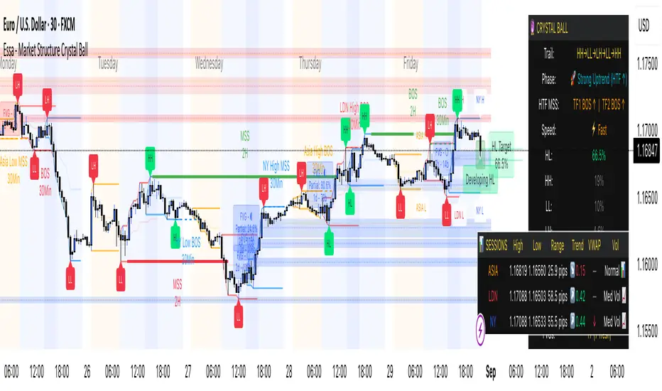
EAOBS by MIGVersion 1
1. Strategy Overview Objective: Capitalize on breakout movements in Ethereum (ETH) price after the Asian open pre-market session (7:00 PM–7:59 PM EST) by identifying high and low prices during the session and trading breakouts above the high or below the low.
Timeframe: Any (script is timeframe-agnostic, but align with session timing).
Session: Pre-market session (7:00 PM–7:59 PM EST, adjustable for other time zones, e.g., 12:00 AM–12:59 AM GMT).
Risk-Reward Ratios (R:R): Targets range from 1.2:1 to 5.2:1, with a fixed stop loss.
Instrument: Ethereum (ETH/USD or ETH-based pairs).
2. Market Setup Session Monitoring: Monitor ETH price action during the pre-market session (7:00 PM–7:59 PM EST), which aligns with the Asian market open (e.g., 9:00 AM–9:59 AM JST).
The script tracks the highest high and lowest low during this session.
Breakout Triggers: Buy Signal: Price breaks above the session’s high after the session ends (7:59 PM EST).
Sell Signal: Price breaks below the session’s low after the session ends.
Visualization: The session is highlighted on the chart with a white background.
Horizontal lines are drawn at the session’s high and low, extended for 30 bars, along with take-profit (TP) and stop-loss (SL) levels.
3. Entry Rules Long (Buy) Entry: Enter a long position when the price breaks above the session’s high price after 7:59 PM EST.
Entry price: Just above the session high (e.g., add a small buffer, like 0.1–0.5%, to avoid false breakouts, depending on volatility).
Short (Sell) Entry: Enter a short position when the price breaks below the session’s low price after 7:59 PM EST.
Entry price: Just below the session low (e.g., subtract a small buffer, like 0.1–0.5%).
Confirmation: Use a candlestick close above/below the breakout level to confirm the entry.
Optionally, add volume confirmation or a momentum indicator (e.g., RSI or MACD) to filter out weak breakouts.
Position Size: Calculate position size based on risk tolerance (e.g., 1–2% of account per trade).
Risk is determined by the stop-loss distance (10 points, as defined in the script).
4. Exit Rules Take-Profit Levels (in points, based on script inputs):TP1: 12 points (1.2:1 R:R).
TP2: 22 points (2.2:1 R:R).
TP3: 32 points (3.2:1 R:R).
TP4: 42 points (4.2:1 R:R).
TP5: 52 points (5.2:1 R:R).
Example for Long: If session high is 3000, TP levels are 3012, 3022, 3032, 3042, 3052.
Example for Short: If session low is 2950, TP levels are 2938, 2928, 2918, 2908, 2898.
Strategy: Scale out of the position (e.g., close 20% at TP1, 20% at TP2, etc.) or take full profit at a preferred TP level based on market conditions.
Stop-Loss: Fixed at 10 points from the entry.
Long SL: Session high - 10 points (e.g., entry at 3000, SL at 2990).
Short SL: Session low + 10 points (e.g., entry at 2950, SL at 2960).
Trailing Stop (Optional):After reaching TP2 or TP3, consider trailing the stop to lock in profits (e.g., trail by 10–15 points below the current price).
5. Risk Management per Trade: Limit risk to 1–2% of your trading account per trade.
Calculate position size: Account Size × Risk % ÷ (Stop-Loss Distance × ETH Price per Point).
Example: $10,000 account, 1% risk = $100. If SL = 10 points and 1 point = $1, position size = $100 ÷ 10 = 0.1 ETH.
Daily Risk Limit: Cap daily losses at 3–5% of the account to avoid overtrading.
Maximum Exposure: Avoid taking both long and short positions simultaneously unless using separate accounts or strategies.
Volatility Consideration: Adjust position size during high-volatility periods (e.g., major news events like Ethereum upgrades or macroeconomic announcements).
6. Trade Management Monitoring :Watch for breakouts after 7:59 PM EST.
Monitor price action near TP and SL levels using alerts or manual checks.
Trade Duration: Breakout lines extend for 30 bars (script parameter). Close trades if no TP or SL is hit within this period, or reassess based on market conditions.
Adjustments: If the market shows strong momentum, consider holding beyond TP5 with a trailing stop.
If the breakout fails (e.g., price reverses before TP1), exit early to minimize losses.
7. Additional Considerations Market Conditions: The 7:00 PM–7:59 PM EST session aligns with the Asian market open (e.g., Tokyo Stock Exchange open at 9:00 AM JST), which may introduce higher volatility due to Asian trading activity.
Avoid trading during low-liquidity periods or extreme volatility (e.g., major crypto news).
Check for upcoming events (e.g., Ethereum network upgrades, ETF decisions) that could impact price.
Backtesting: Test the strategy on historical ETH data using the session high/low breakouts for the 7:00 PM–7:59 PM EST window to validate performance.
Adjust TP/SL levels based on backtest results if needed.
Broker and Fees: Use a low-fee crypto exchange (e.g., Binance, Kraken, Coinbase Pro) to maximize R:R.
Account for trading fees and slippage in your position sizing.
Time zone Adjustment: Adjust session time input for your time zone (e.g., "0000-0059" for GMT).
Ensure your trading platform’s clock aligns with the script’s time zone (default: America/New_York).
8. Example Trade Scenario: Session (7:00 PM–7:59 PM EST) records a high of 3050 and a low of 3000.
Long Trade: Entry: Price breaks above 3050 (e.g., enter at 3051).
TP Levels: 3063 (TP1), 3073 (TP2), 3083 (TP3), 3093 (TP4), 3103 (TP5).
SL: 3040 (3050 - 10).
Position Size: For a $10,000 account, 1% risk = $100. SL = 11 points ($11). Size = $100 ÷ 11 = ~0.09 ETH.
Short Trade: Entry: Price breaks below 3000 (e.g., enter at 2999).
TP Levels: 2987 (TP1), 2977 (TP2), 2967 (TP3), 2957 (TP4), 2947 (TP5).
SL: 3010 (3000 + 10).
Position Size: Same as above, ~0.09 ETH.
Execution: Set alerts for breakouts, enter with limit orders, and monitor TPs/SL.
9. Tools and Setup Platform: Use TradingView to implement the Pine Script and visualize breakout levels.
Alerts: Set price alerts for breakouts above the session high or below the session low after 7:59 PM EST.
Set alerts for TP and SL levels.
Chart Settings: Use a 1-minute or 5-minute chart for precise session tracking.
Overlay the script to see high/low lines, TP levels, and SL levels.
Optional Indicators: Add RSI (e.g., avoid overbought/oversold breakouts) or volume to confirm breakouts.
10. Risk Warnings Crypto Volatility: ETH is highly volatile; unexpected news can cause rapid price swings.
False Breakouts: Breakouts may fail, especially in low-volume sessions. Use confirmation signals.
Leverage: Avoid high leverage (e.g., >5x) to prevent liquidation during volatile moves.
Session Accuracy: Ensure correct session timing for your time zone to avoid misaligned entries.
11. Performance Tracking Journaling :Record each trade’s entry, exit, R:R, and outcome.
Note market conditions (e.g., trending, ranging, news-driven).
Review: Weekly: Assess win rate, average R:R, and adherence to the plan.
Monthly: Adjust TP/SL or session timing based on performance.
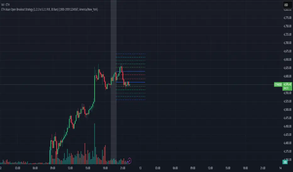
X OROverview
Designed to plot hourly opening ranges (ORs) on an intraday chart. It primarily serves as a trading tool for assessing market direction and potential trading opportunities by analyzing price action relative to key OHLC (Open, High, Low, Close) levels within each hourly range.
The code provided is for each hour sessions from 2:00 AM to 3:00 PM for a complete session-based framework. In addition there is the RTH open range
Purpose
The core purpose of this indicator is to:
✅ Define each hourly range (based on the session’s opening bar) by recording the high and low of that range.
✅ Extend this range into the following bars for visual reference — serving as dynamic support and resistance zones.
✅ Monitor price action relative to each hourly OR, helping traders evaluate market direction and structure trades using concepts like:
Breakouts above/below the OR high/low.
Rejections or consolidations within the OR.
Continuation or reversal signals tied to each OR.
Key Features
The script marks the first bar of the session as the OR session start.
During this bar, it initializes:
Opening price
Session high
Session low
These levels form the initial range.
🔹 Dynamic Range Tracking
Throughout the one-minute OR session:
The highest and lowest prices are updated in real time, capturing intra-hour volatility.
A visual background box is drawn to highlight the OR range on the chart.
🔹 Range Extension
The script defines an extended session period after the initial OR (e.g., 2:00 AM-2:45 AM for the 2:00 AM session).
During this extension period:
The box persists on the chart, providing a contextual zone that traders can use as a dynamic support/resistance area.
🔹 Visual Representation
Transparent colored boxes highlight each session’s OR visually on the chart.
These boxes help traders easily identify whether price is trading:
Inside the OR
Breaking above the high (potential bullish continuation)
Breaking below the low (potential bearish continuation)
Application in Trading
🔍 Trading the Opening Range Breakout
Traders often use the OR high and low as breakout triggers. For example:
A price break above the OR high may signal bullish momentum.
A break below the OR low may signal bearish momentum.
⚖️ Support and Resistance
Even if breakouts fail, the OR can act as a pivot zone — offering areas for:
Stop placements
Target levels
Entry confirmations for fade trades or mean reversion strategies.
🕒 Session Awareness
By defining each hour’s OR individually (from 2:00 AM to 3:00 PM), traders can:
Analyze price behavior within each session.
Recognize when liquidity or volatility increases (e.g. around overlapping sessions like London open or New York open).
Summary
This Pine Script indicator provides a powerful framework for visualizing and trading hourly opening ranges. It enhances intraday analysis by:
Structuring price action within hourly boxes.
Highlighting key price levels relative to OHLC concepts.
Helping traders make more informed decisions by assessing price behavior around these critical ranges.

Intraday Pivot Highs & Lows (Asia London NY)Intraday Pivot Highs & Lows (Asia London NY)
Script Description
This TradingView indicator is optimized for Forex, scalping, intraday, and day trading strategies. It accurately plots Pivot Points and levels, high/low, support and resistance levels. These are clearly identified to aid the trader during killzone sessions and session opens. Ideal for scalp trading, intraday sessions, and leveraging SMT (Smart Money Techniques). Utilize these Price Levels effectively during London Open, NY Open, and the Asia Session, utilizing Market Structure to pinpoint key levels and reversal zones for successful trading. Improve your Trade Setups, recognize reliable Chart Patterns, identify critical Price Pivots, and trade confidently off Institutional Levels.
This script marks the intraday pivot highs, lows and midpoints retracement levels for
Asia
London
New York
It also plots the previous day's high, low, midpoint, and 0.618 Fibonacci retracement levels, providing traders with critical price reference points for making intraday trading decisions.
Originality & Usefulness
This indicator uniquely integrates pivot calculations across three major Forex sessions (Asia, London, NY), clearly delineating session boundaries.
It enhances visibility by using distinct styling
solid for New York
dashed for London
dotted lines for Asia
And colour co-ordinated labeling, improving traders' ability to identify important intraday price action zones efficiently. Unlike standard pivot indicators, this script emphasizes session-specific trading dynamics.
### Key Features ###
Session-Based Levels: Automatically plots high, low, midpoint, and Fibonacci (.618) levels for each major session (Asia, London, NY).
Distinct Visual Cues: Lines and labels use session-specific styles and colors to easily differentiate between sessions.
Previous Day Reference: Clearly plots and labels yesterday's high, low, midpoint, and Fibonacci levels.
Flexible Visibility: Traders can set timeframe visibility to maintain clean charts on higher timeframes.
### How It Works
At the start of next day's session, previous session lines are cleared, ensuring the chart remains uncluttered.
High, low, midpoint, and Fibonacci retracement levels (.618) are dynamically calculated and displayed at the close of each session.
All session levels remain visible until the start of the next respective session, providing continuous actionable insights.
Trading Application:
Session highs and lows act as strong intraday support and resistance zones.
Midpoints and Fibonacci levels are effective for identifying potential reversal zones and retracements.
Daily levels provide a broader context, useful for gauging intraday volatility and range.
### Limitations and Considerations ##
Best used on liquid assets with clear session-based price action, such as Forex major pairs, if used on indexes make sure they contain 24 hour price action not just New York session.
This indicator is designed to streamline intraday trading by clearly marking essential pivot points and session-based levels, significantly improving traders' market context and decision-making accuracy. Can be used to enhance SMT decision making when scalping killzones.
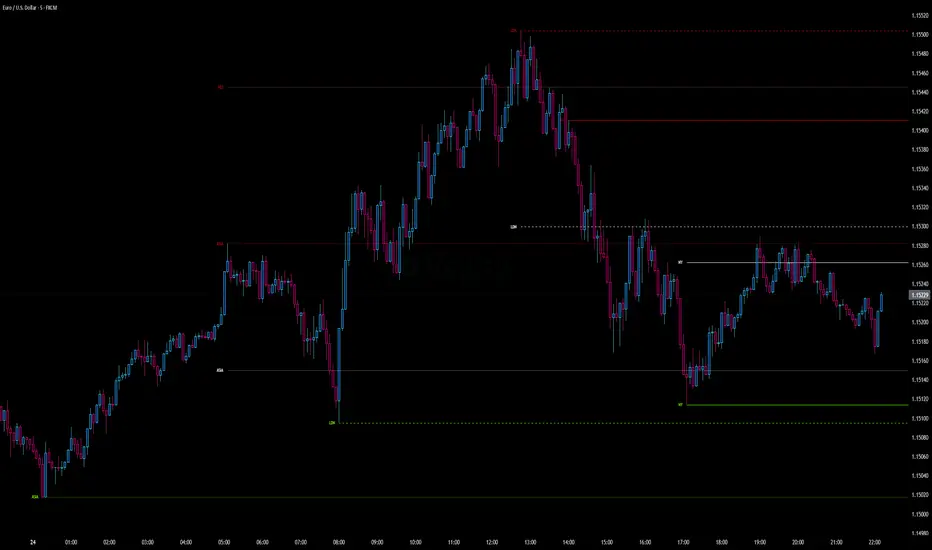
Globex time (New York Time)This indicator is designed to highlight and analyze price movements within the Globex session. Primarily geared toward the Globex Trap trading strategy, this tool visually identifies the session's high and low prices, allowing traders to better assess price action during extended hours. Here’s a comprehensive breakdown of its features and functionality:
Purpose
The "Globex Time (New York Time)" indicator tracks price levels during the Globex trading session, providing a clear view of overnight market activity. This session, typically running from 6 p.m. ET (18:00) until the following morning at 8:30 a.m. ET, is a critical period where significant market positioning can occur before the regular session opens. In the Globex Trap strategy, the session high and low are essential levels, as price movements around these areas often indicate potential support, resistance, or reversal zones, which traders use to set up entries or exits when the regular trading session begins.
Key Features
Customizable Session Start and End Times
The indicator allows users to specify the exact start and end times of the Globex session in New York time. The default settings are:
Start: 6 p.m. ET (18:00)
End: 8:30 a.m. ET
These settings can be adjusted to align with specific market hours or personal preferences.
Session High and Low Identification
Throughout the defined session, the indicator dynamically calculates and tracks:
Session High: The highest price reached within the session.
Session Low: The lowest price reached within the session.
These levels are essential for the Globex Trap strategy, as price action around them can indicate likely breakout or reversal points when regular trading resumes.
Vertical Lines for Session Start and End
The indicator draws vertical lines at both the session start and end times:
Session Start Line: A solid line marking the exact beginning of the Globex session.
Session End Line: A similar vertical line marking the session’s conclusion.
Both lines are customizable in terms of color and thickness, making it easy to distinguish the session boundaries visually on the chart.
Horizontal Lines for Session High and Low
At the end of the session, the indicator plots horizontal lines representing the Globex session's high and low levels. Users can customize these lines:
Color: Define specific colors for the session high (default: red) and session low (default: green) to easily differentiate them.
Line Style: Options to set the line style (solid, dashed, or dotted) provide flexibility for visual preferences and chart organization.
Automatic Reset for Daily Tracking
To adapt to the next trading day, the indicator resets the session high and low data once the current session ends. This reset prepares it to start tracking new levels at the beginning of the next session without manual intervention.
Practical Application in the Globex Trap Strategy
In the Globex Trap strategy, traders are primarily interested in price behavior around the high and low levels established during the overnight session. Common applications of this indicator for this strategy include:
Breakout Trades: Watching for price to break above the Globex high or below the Globex low, indicating potential momentum in the breakout direction.
Reversal Trades: Monitoring for failed breakouts or traps where price tests and rejects the Globex high or low, suggesting a reversal as liquidity is trapped in these zones.
Support and Resistance Zones: Using the session high and low as key support and resistance levels during the regular trading session, with potential entry or exit points when price approaches these areas.
Additional Configuration Options
Vertical Line Color and Width: Define the color and thickness of the vertical session start and end lines to match your chart’s theme.
Upper and Lower Line Colors and Styles: Customize the appearance of the session high and low horizontal lines by setting color and line style (solid, dashed, or dotted), making it easy to distinguish these critical levels from other chart markings.
Summary
This indicator is a valuable tool for traders implementing the Globex Trap strategy. It visually segments the Globex session and marks essential price levels, helping traders analyze market behavior overnight. Through its customizable options and clear visual representation, it simplifies tracking overnight price activity and identifying strategic levels for potential trade setups during the regular session.

ICT Master Suite [Trading IQ]Hello Traders!
We’re excited to introduce the ICT Master Suite by TradingIQ, a new tool designed to bring together several ICT concepts and strategies in one place.
The Purpose Behind the ICT Master Suite
There are a few challenges traders often face when using ICT-related indicators:
Many available indicators focus on one or two ICT methods, which can limit traders who apply a broader range of ICT related techniques on their charts.
There aren't many indicators for ICT strategy models, and we couldn't find ICT indicators that allow for testing the strategy models and setting alerts.
Many ICT related concepts exist in the public domain as indicators, not strategies! This makes it difficult to verify that the ICT concept has some utility in the market you're trading and if it's worth trading - it's difficult to know if it's working!
Some users might not have enough chart space to apply numerous ICT related indicators, which can be restrictive for those wanting to use multiple ICT techniques simultaneously.
The ICT Master Suite is designed to offer a comprehensive option for traders who want to apply a variety of ICT methods. By combining several ICT techniques and strategy models into one indicator, it helps users maximize their chart space while accessing multiple tools in a single slot.
Additionally, the ICT Master Suite was developed as a strategy . This means users can backtest various ICT strategy models - including deep backtesting. A primary goal of this indicator is to let traders decide for themselves what markets to trade ICT concepts in and give them the capability to figure out if the strategy models are worth trading!
What Makes the ICT Master Suite Different
There are many ICT-related indicators available on TradingView, each offering valuable insights. What the ICT Master Suite aims to do is bring together a wider selection of these techniques into one tool. This includes both key ICT methods and strategy models, allowing traders to test and activate strategies all within one indicator.
Features
The ICT Master Suite offers:
Multiple ICT strategy models, including the 2022 Strategy Model and Unicorn Model, which can be built, tested, and used for live trading.
Calculation and display of key price areas like Breaker Blocks, Rejection Blocks, Order Blocks, Fair Value Gaps, Equal Levels, and more.
The ability to set alerts based on these ICT strategies and key price areas.
A comprehensive, yet practical, all-inclusive ICT indicator for traders.
Customizable Timeframe - Calculate ICT concepts on off-chart timeframes
Unicorn Strategy Model
2022 Strategy Model
Liquidity Raid Strategy Model
OTE (Optimal Trade Entry) Strategy Model
Silver Bullet Strategy Model
Order blocks
Breaker blocks
Rejection blocks
FVG
Strong highs and lows
Displacements
Liquidity sweeps
Power of 3
ICT Macros
HTF previous bar high and low
Break of Structure indications
Market Structure Shift indications
Equal highs and lows
Swings highs and swing lows
Fibonacci TPs and SLs
Swing level TPs and SLs
Previous day high and low TPs and SLs
And much more! An ongoing project!
How To Use
Many traders will already be familiar with the ICT related concepts listed above, and will find using the ICT Master Suite quite intuitive!
Despite this, let's go over the features of the tool in-depth and how to use the tool!
The image above shows the ICT Master Suite with almost all techniques activated.
ICT 2022 Strategy Model
The ICT Master suite provides the ability to test, set alerts for, and live trade the ICT 2022 Strategy Model.
The image above shows an example of a long position being entered following a complete setup for the 2022 ICT model.
A liquidity sweep occurs prior to an upside breakout. During the upside breakout the model looks for the FVG that is nearest 50% of the setup range. A limit order is placed at this FVG for entry.
The target entry percentage for the range is customizable in the settings. For instance, you can select to enter at an FVG nearest 33% of the range, 20%, 66%, etc.
The profit target for the model generally uses the highest high of the range (100%) for longs and the lowest low of the range (100%) for shorts. Stop losses are generally set at 0% of the range.
The image above shows the short model in action!
Whether you decide to follow the 2022 model diligently or not, you can still set alerts when the entry condition is met.
ICT Unicorn Model
The image above shows an example of a long position being entered following a complete setup for the ICT Unicorn model.
A lower swing low followed by a higher swing high precedes the overlap of an FVG and breaker block formed during the sequence.
During the upside breakout the model looks for an FVG and breaker block that formed during the sequence and overlap each other. A limit order is placed at the nearest overlap point to current price.
The profit target for this example trade is set at the swing high and the stop loss at the swing low. However, both the profit target and stop loss for this model are configurable in the settings.
For Longs, the selectable profit targets are:
Swing High
Fib -0.5
Fib -1
Fib -2
For Longs, the selectable stop losses are:
Swing Low
Bottom of FVG or breaker block
The image above shows the short version of the Unicorn Model in action!
For Shorts, the selectable profit targets are:
Swing Low
Fib -0.5
Fib -1
Fib -2
For Shorts, the selectable stop losses are:
Swing High
Top of FVG or breaker block
The image above shows the profit target and stop loss options in the settings for the Unicorn Model.
Optimal Trade Entry (OTE) Model
The image above shows an example of a long position being entered following a complete setup for the OTE model.
Price retraces either 0.62, 0.705, or 0.79 of an upside move and a trade is entered.
The profit target for this example trade is set at the -0.5 fib level. This is also adjustable in the settings.
For Longs, the selectable profit targets are:
Swing High
Fib -0.5
Fib -1
Fib -2
The image above shows the short version of the OTE Model in action!
For Shorts, the selectable profit targets are:
Swing Low
Fib -0.5
Fib -1
Fib -2
Liquidity Raid Model
The image above shows an example of a long position being entered following a complete setup for the Liquidity Raid Modell.
The user must define the session in the settings (for this example it is 13:30-16:00 NY time).
During the session, the indicator will calculate the session high and session low. Following a “raid” of either the session high or session low (after the session has completed) the script will look for an entry at a recently formed breaker block.
If the session high is raided the script will look for short entries at a bearish breaker block. If the session low is raided the script will look for long entries at a bullish breaker block.
For Longs, the profit target options are:
Swing high
User inputted Lib level
For Longs, the stop loss options are:
Swing low
User inputted Lib level
Breaker block bottom
The image above shows the short version of the Liquidity Raid Model in action!
For Shorts, the profit target options are:
Swing Low
User inputted Lib level
For Shorts, the stop loss options are:
Swing High
User inputted Lib level
Breaker block top
Silver Bullet Model
The image above shows an example of a long position being entered following a complete setup for the Silver Bullet Modell.
During the session, the indicator will determine the higher timeframe bias. If the higher timeframe bias is bullish the strategy will look to enter long at an FVG that forms during the session. If the higher timeframe bias is bearish the indicator will look to enter short at an FVG that forms during the session.
For Longs, the profit target options are:
Nearest Swing High Above Entry
Previous Day High
For Longs, the stop loss options are:
Nearest Swing Low
Previous Day Low
The image above shows the short version of the Silver Bullet Model in action!
For Shorts, the profit target options are:
Nearest Swing Low Below Entry
Previous Day Low
For Shorts, the stop loss options are:
Nearest Swing High
Previous Day High
Order blocks
The image above shows indicator identifying and labeling order blocks.
The color of the order blocks, and how many should be shown, are configurable in the settings!
Breaker Blocks
The image above shows indicator identifying and labeling order blocks.
The color of the breaker blocks, and how many should be shown, are configurable in the settings!
Rejection Blocks
The image above shows indicator identifying and labeling rejection blocks.
The color of the rejection blocks, and how many should be shown, are configurable in the settings!
Fair Value Gaps
The image above shows indicator identifying and labeling fair value gaps.
The color of the fair value gaps, and how many should be shown, are configurable in the settings!
Additionally, you can select to only show fair values gaps that form after a liquidity sweep. Doing so reduces "noisy" FVGs and focuses on identifying FVGs that form after a significant trading event.
The image above shows the feature enabled. A fair value gap that occurred after a liquidity sweep is shown.
Market Structure
The image above shows the ICT Master Suite calculating market structure shots and break of structures!
The color of MSS and BoS, and whether they should be displayed, are configurable in the settings.
Displacements
The images above show indicator identifying and labeling displacements.
The color of the displacements, and how many should be shown, are configurable in the settings!
Equal Price Points
The image above shows the indicator identifying and labeling equal highs and equal lows.
The color of the equal levels, and how many should be shown, are configurable in the settings!
Previous Custom TF High/Low
The image above shows the ICT Master Suite calculating the high and low price for a user-defined timeframe. In this case the previous day’s high and low are calculated.
To illustrate the customizable timeframe function, the image above shows the indicator calculating the previous 4 hour high and low.
Liquidity Sweeps
The image above shows the indicator identifying a liquidity sweep prior to an upside breakout.
The image above shows the indicator identifying a liquidity sweep prior to a downside breakout.
The color and aggressiveness of liquidity sweep identification are adjustable in the settings!
Power Of Three
The image above shows the indicator calculating Po3 for two user-defined higher timeframes!
Macros
The image above shows the ICT Master Suite identifying the ICT macros!
ICT Macros are only displayable on the 5 minute timeframe or less.
Strategy Performance Table
In addition to a full-fledged TradingView backtest for any of the ICT strategy models the indicator offers, a quick-and-easy strategy table exists for the indicator!
The image above shows the strategy performance table in action.
Keep in mind that, because the ICT Master Suite is a strategy script, you can perform fully automatic backtests, deep backtests, easily add commission and portfolio balance and look at pertinent metrics for the ICT strategies you are testing!
Lite Mode
Traders who want the cleanest chart possible can toggle on “Lite Mode”!
In Lite Mode, any neon or “glow” like effects are removed and key levels are marked as strict border boxes. You can also select to remove box borders if that’s what you prefer!
Settings Used For Backtest
For the displayed backtest, a starting balance of $1000 USD was used. A commission of 0.02%, slippage of 2 ticks, a verify price for limit orders of 2 ticks, and 5% of capital investment per order.
A commission of 0.02% was used due to the backtested asset being a perpetual future contract for a crypto currency. The highest commission (lowest-tier VIP) for maker orders on many exchanges is 0.02%. All entered positions take place as maker orders and so do profit target exits. Stop orders exist as stop-market orders.
A slippage of 2 ticks was used to simulate more realistic stop-market orders. A verify limit order settings of 2 ticks was also used. Even though BTCUSDT.P on Binance is liquid, we just want the backtest to be on the safe side. Additionally, the backtest traded 100+ trades over the period. The higher the sample size the better; however, this example test can serve as a starting point for traders interested in ICT concepts.
Community Assistance And Feedback
Given the complexity and idiosyncratic applications of ICT concepts amongst its proponents, the ICT Master Suite’s built-in strategies and level identification methods might not align with everyone's interpretation.
That said, the best we can do is precisely define ICT strategy rules and concepts to a repeatable process, test, and apply them! Whether or not an ICT strategy is trading precisely how you would trade it, seeing the model in action, taking trades, and with performance statistics is immensely helpful in assessing predictive utility.
If you think we missed something, you notice a bug, have an idea for strategy model improvement, please let us know! The ICT Master Suite is an ongoing project that will, ideally, be shaped by the community.
A big thank you to the @PineCoders for their Time Library!
Thank you!

AMDX/XAMD indicatorThe AMDX/XAMD indicator is designed to highlight specific trading sessions on the chart using distinct colors and optional vertical lines. Users can choose between two session types, AMDX or XAMD, and customize the visual appearance of the sessions. This tool is particularly useful for traders who want to analyze market behavior during different trading periods.
Meaning of AMDX:
A: Accumulation
M: Manipulation
D: Distribution
X: Continuation Or Reversal
Features:
Session Highlighting:
AMDX Sessions: Split into four segments - A, M, D, X.
XAMD Sessions: Split into four segments - X, A, M, D.
Customizable Colors:
Choose individual colors for each session (A, M, D, X).
Adjust the transparency of the session boxes for better visual integration with the chart.
Drawing Styles:
Box Style: Draws colored boxes around the session ranges.
Line Style: Draws vertical lines at session start and end times.
Vertical Lines:
Option to enable or disable vertical lines at session boundaries.
Customizable line style: Solid, Dotted, or Dashed.
Session Labels:
Automatically labels each session for easy identification.
Customization Options:
Session Type: Select between AMDX and XAMD session types.
Colors: Set custom colors for each session and vertical lines.
Border Width: Adjust the width of the session box borders.
Transparency: Control the transparency level of the session boxes.
Drawing Style: Choose between Box and Line styles for session representation.
Vertical Lines: Enable or disable vertical lines and select the line style.
How It Works:
The indicator calculates the start and end times for each session based on the selected session type (AMDX or XAMD). It then draws either boxes or lines to highlight these sessions on the chart. The indicator also includes options to draw vertical lines at the session boundaries and labels each session with a corresponding letter (A, M, D, X).
Use Cases:
Market Session Analysis: Easily identify and analyze market behavior during different trading sessions.
Intraday Trading: Helps intraday traders to focus on specific time segments of the trading day.
Visual Segmentation: Provides a clear visual segmentation of the trading day, aiding in better decision-making.
Times for AMDX/XAMD session:
A Session: 18:00 (previous day) to 03:00 (current day)
M Session: 03:00 to 09:00
D Session: 09:00 to 12:00
X Session: 12:00 to 18:00
Time for the XAMD session :
X Session: 18:00 (previous day) to 00:00 (current day)
A Session: 00:00 to 09:00
M Session: 09:00 to 12:00
D Session: 12:00 to 18:00
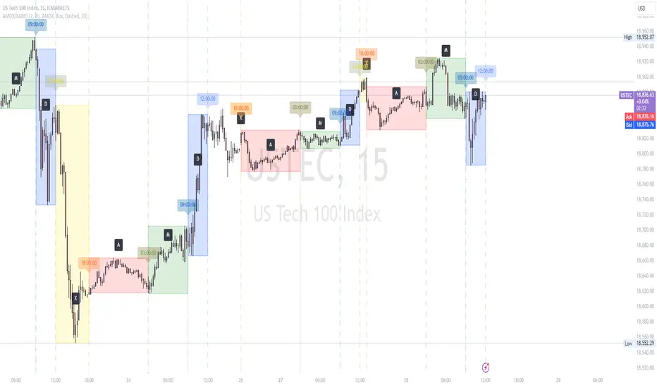
Session candles & reversals / quantifytools— Overview
Like traditional candles, session based candles are a visualization of open, high, low and close values, but based on session time periods instead of typical timeframes such as daily or weekly. Session candles are formed by fetching price at session start (open), highest price during session (high), lowest price during session (low) and price at session end (close). On top of candles, session based moving average is formed and session reversals detected. Session reversals are also backtested, using win rate and magnitude metrics to better understand what to expect from session reversals and which ones have historically performed the best.
By default, following session time periods are used:
Session #1: London (08:00 - 17:00, UTC)
Session #2: New York (13:00 - 22:00, UTC)
Session #3: Sydney (21:00 - 06:00, UTC)
Session #4: Tokyo (00:00 - 09:00, UTC)
Session time periods can be changed via input menu.
— Reversals
Session reversals are patterns that show a rapid change in direction during session. These formations are more familiarly known as wicks or engulfing candles. Following criteria must be met to qualify as a session reversal:
Wick up:
Lower high, lower low, close >= 65% of session range (0% being the very low, 100% being the very high) and open >= 40% of session range.
Wick down:
Higher high, higher low, close <= 35% of session range and open <= 60% of session range.
Engulfing up:
Higher high, lower low, close >= 65% of session range.
Engulfing down:
Higher high, lower low, close <= 35% of session range.
Session reversals are always based on prior corresponding session , e.g. to qualify as a NY session engulfing up, NY session must have a higher high and lower low relative to prior NY session , not just any session that has taken place in between. Session reversals should be viewed the same way wicks/engulfing formations are viewed on traditional timeframe based candles. Essentially, wick reversals (light green/red labels) tell you most of the motion during session was reversed. Engulfing reversals (dark green/red labels) on the other hand tell you all of the motion was reversed and new direction set.
— Backtesting
Session reversals are backtested using win rate and magnitude metrics. A session reversal is considered successful when next corresponding session closes higher/lower than session reversal close . Win rate is formed by dividing successful session reversal count with total reversal count, e.g. 5 successful reversals up / 10 reversals up total = 50% win rate. Win rate tells us what are the odds (historically) of session reversal producing a clean supporting move that was persistent enough to close that way too.
When a session reversal is successful, its magnitude is measured using percentage increase/decrease from session reversal close to next corresponding session high/low . If NY session closes higher than prior NY session that was a reversal up, the percentage increase from prior session close (reversal close) to current session high is measured. If NY session closes lower than prior NY session that was a reversal down, the percentage decrease from prior session close to current session low is measured.
Average magnitude is formed by dividing all percentage increases/decreases with total reversal count, e.g. 10 total reversals up with 1% increase each -> 10% net increase from all reversals -> 10% total increase / 10 total reversals up = 1% average magnitude. Magnitude metric supports win rate by indicating the depth of successful session reversal moves.
To better understand the backtesting calculations and more importantly to verify their validity, backtesting visuals for each session can be plotted on the chart:
All backtesting results are shown in the backtesting panel on top right corner, with highest win rates and magnitude metrics for both reversals up and down marked separately. Note that past performance is not a guarantee of future performance and session reversals as they are should not be viewed as a complete strategy for long/short plays. Always make sure reversal count is sufficient to draw reliable conclusions of performance.
— Session moving average
Users can form a session based moving average with their preferred smoothing method (SMA , EMA , HMA , WMA , RMA) and length, as well as choose which sessions to include in the moving average. For example, a moving average based on New York and Tokyo sessions can be formed, leaving London and Sydney completely out of the calculation.
— Visuals
By default, script hides your candles/bars, although in the case of candles borders will still be visible. Switching to bars/line will make your regular chart visuals 100% hidden. This setting can be turned off via input menu. As some sessions overlap, each session candle can be separately offsetted forward, clearing the overlaps. Users can also choose which session candles to show/hide.
Session periods can be highlighted on the chart as a background color, applicable to only session candles that are activated. By default, session reversals are referred to as L (London), N (New York), S (Sydney) and T (Tokyo) in both reversal labels and backtesting table. By toggling on "Numerize sessions", these will be replaced with 1, 2, 3 and 4. This will be helpful when using a custom session that isn't any of the above.
Visual settings example:
Session candles are plotted in two formats, using boxes and lines as well as plotcandle() function. Session candles constructed using boxes and lines will be clear and much easier on the eyes, but will apply only to first 500 bars due to Tradingview related limitations. Rest of the session candles go back indefinitely, but won't be as clean:
All colors can be customized via input menu.
— Timeframe & session time period considerations
As a rule of thumb, session candles should be used on timeframes at or below 1H, as higher timeframes might not match with session period start/end, leading to incorrect plots. Using 1 hour timeframe will bring optimal results as greatest amount historical data is available without sacrificing accuracy of OHLC values. If you are using a custom session that is not based on hourly period (e.g. 08:00 - 15:00 vs. 08.00 - 15.15) make sure you are using a timeframe that allows correct plots.
Session time periods applied by default are rough estimates and might be out of bounds on some charts, like NYSE listed equities. This is rarely a problem on assets that have extensive trading hours, like futures or cryptocurrency. If a session is out of bounds (asset isn't traded during the set session time period) the script won't plot given session candle and its backtesting metrics will be NA. This can be fixed by changing the session time periods to match with given asset trading hours, although you will have to consider whether or not this defeats the purpose of having candles based on sessions.
— Practical guide
Whether based on traditional timeframes or sessions, reversals should always be considered as only one piece of evidence of price turning. Never react to them without considering other factors that might support the thesis, such as levels and multi-timeframe analysis. In short, same basic charting principles apply with session candles that apply with normal candles. Use discretion.
Example #1 : Focusing efforts on session reversals at distinct support/resistance levels
A reversal against a level holds more value than a reversal by itself, as you know it's a placement where liquidity can be expected. A reversal serves as a confirming reaction for this expectation.
Example #2 : Focusing efforts on highest performing reversals and avoiding poorly performing ones
As you have data backed evidence of session reversal performance, it makes sense to focus your efforts on the ones that perform best. If some session reversal is clearly performing poorly, you would want to avoid it, since there's nothing backing up its validity.
Example #3 : Reversal clusters
Two is better than one, three is better than two and so on. If there are rapid changes in direction within multiple sessions consecutively, there's heavier evidence of a dynamic shift in price. In such case, it makes sense to hold more confidence in price halting/turning.

Session Levels - Ultimate Range IndicatorSession Levels - Ultimate Range Indicator
Primarily developed for trading the E-MINI Futures Markets like NQ or ES from the CME Group,
but also more than suitable for Crypto or other instruments.
This indicator highlights the chosen session, which can be Globex, Asian, London and New York.
It plots the important levels and also renders the Opening Range as it forms (a.k.a. Initial Balance).
After the 1st hour Opening Range is finished, it can plot the Standard Deviations / Projections.
See below for a complete feature list.
All Opening Ranges on chart and for the New York session the Range Projections are turned on:
s3.tradingview.com
How to use (example):
If you are trading the Nasdaq Futures (NQ!)
Enable the Globex Overnight session. Basically in the Futures Market, the Globex session is everything outside of US trading hours of Stocks. This draws the important overnight levels, like the Low, 25%, 50%, 75% and the High.
Enable the New York Session with Levels and Opening Range. Generally, 70% of the time the 1st hour will put a Low or High of the day.
If the price is trading above the Globex Low, most likely the Low of the Day is formed and the price target for the day will be 1.5x Standard Deviation and 2x Standard Deviation.
[*} Deviation of the Initial Balance depends on the volume ad overall market structure.
** This is not financial advice or any guarantee **
Features:
Show each Session Highlighted on Intraday chart in it's own color (each session can be turned off and has customizable times and color)
Show Line Levels of each session: Low, 25%, 50%, 75% and the High (customizable color)
Show the Opening Range (Initial Balance) of the Asian, London and New York session. Note: NY has more options.
Opening Range is displayed as a box with level lines (customizable color)
Levels are drawn to the end of the NY Cash session (customizable time)
Show IB Standard Deviations 0.5 - 3.0. Calculated from the Opening Range (Initial Balance)
Option to display Higher Timeframe levels: Previous Day Open/Close and Previous Week Open/Close
All level lines and OR boxes size dynamically as the session progresses
Built in Alerts for when price hits key levels. e.g. Alert when price crosses the NY Opening Range High. Or an Alert when the first STDEV is hit.
Option to toggle display of drawings for Today's trading session only, or Show all recent session levels. This keeps the chart clean or not.
Extras:
The NY Opening Range also has a 50% level line
The NY Opening Bar can be highlighted separately
The Level Lines can have small labels turned on/off. Values are only shown on mouse over to keep a clean chart
Keep in mind:
1) This indicator works on all instruments, but on instruments with limited market hours, your chart setting
has to be set to "Extended Hours" otherwise. For example TSLA on NASDAQ.
2) The Exchange Time Zone for the CME Group is Chicago UTC-6. So the session times you configure in the settings menu are based on that timezone too.
3) Globex opens at 5pm CST and closes when the US session starts 8:30CST.
4) When enabling the Alerts in the Indicator settings, be sure to also create an alarm for this indicator using the Alarm function of Tradingview.
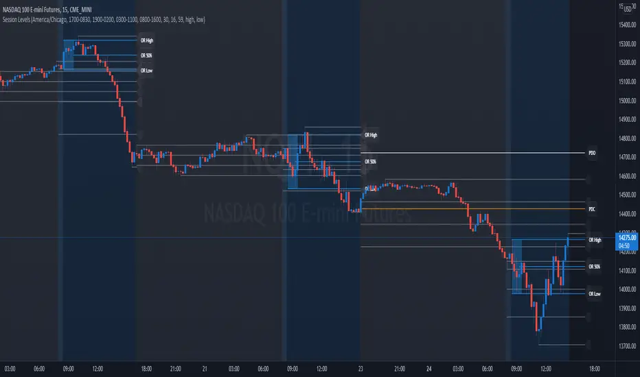
Highlight 6-7 PM (IST) candle + mark H/L (Hourly)📌 Highlight 6–7 PM Candle (IST) + High/Low Lines (No Labels)
This indicator automatically detects the 6:00–7:00 PM candle (IST) on the hourly timeframe and visually marks it on the chart.
It highlights the candle and draws horizontal High and Low levels without any labels—making the chart clean and easy to read.
✅ Features
Highlights the 6–7 PM hourly candle (timezone adjustable: IST/UTC/Exchange).
Draws high & low horizontal lines from the target candle.
Option to extend the lines for a selected number of bars.
Optional restriction to only show on 1-hour timeframe.
Clean design — no labels, no clutter.
🛠️ Inputs
Timezone (default: Asia/Kolkata)
Target Hour (default: 18 = 6 PM)
Highlight Color
High/Low Line Colors
Line Extension Length
Enable/Disable Hourly-only Mode
🎯 Use Case
Useful for traders who track post-market candles, volatility behavior, range levels, or want to build intraday strategies based on evening session highs/lows.

Global Sessions by Back Ground ColorGlobal Sessions Background Color Indicator
This free TradingView tool visually highlights major global trading sessions directly on your chart using clean, professional color coding. It’s designed to help traders quickly identify periods of high liquidity and overlapping sessions, which often drive volatility and key price movements.
Features:
Session Highlights: Marks Asian, European (London), US (New York), and Overnight sessions with distinct background colors.
Overlap Detection: Special colors for overlapping sessions (e.g., London + New York).
Market Open/Close Alerts: Displays labels for major financial centers when they open or close.
Timezone-Aware: Automatically adjusts to Europe/Amsterdam (modifiable for your needs).
Clean Design: Uses a light, professional color palette for easy chart readability.
Why Use It?
Session timing is critical for spotting breakouts, reversals, and liquidity shifts. This indicator gives traders a clear visual edge without cluttering the chart—perfect for scalpers, day traders, and swing traders.
Completely free for the TradingView community – built by a trader, for traders.
How to Use the Global Sessions Indicator
This indicator automatically highlights major trading sessions on your chart using background colors. It helps you quickly identify when liquidity and volatility are likely to increase.
Color Guide:
Light Sky Blue → Asian Session (Tokyo, Sydney)
Active from 02:00 to 12:00 Amsterdam time. Often quieter but sets early trends.
Light Coral → European Session (London, Frankfurt)
Active from 09:00 to 17:30 Amsterdam time. Brings strong liquidity and trend continuation.
Light Green → US Session (New York, Chicago)
Active from 15:30 to 22:00 Amsterdam time. High volatility, major moves often occur here.
Gold/Yellow → Overnight/Wellington
Active from 23:00 to 02:00 Amsterdam time. Low liquidity, pre-Asia positioning.
Overlap Colors:
Orchid (Pinkish) → Asia + Europe Overlap
Indicates transition from Asia to London—watch for breakouts.
Light Salmon → Europe + US Overlap
The most volatile period of the day—ideal for intraday traders.
Extra Feature:
Labels show market open/close times for major financial centers (e.g., London Open, New York Close).
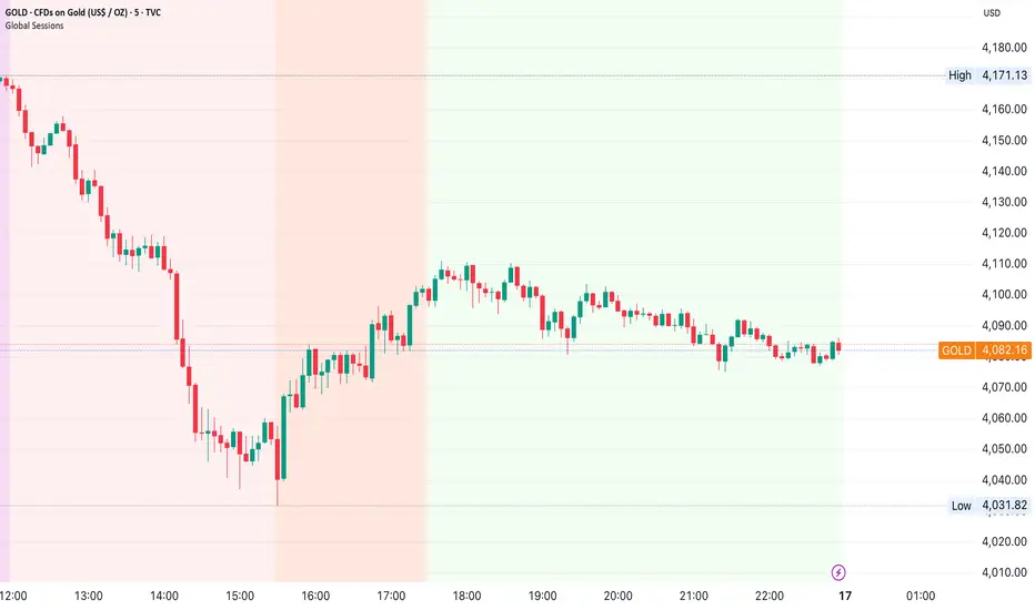
Indian market session on Gift Nifty chartsGift Nifty Market Session Highlighter
This indicator highlights the official Indian market session on Gift Nifty charts — from 9:15 AM to 3:30 PM IST. It shades the background during this time window so traders can instantly identify when the local market is open.
Features:
Marks 9:15 AM to 3:30 PM (IST) session on intraday charts.
Adjustable highlight color and transparency.
Works seamlessly across lower timeframes (1m, 5m, 15m, etc.).
Helps traders align Gift Nifty activity with NSE market hours.
Use Cases:
Quickly distinguish active market hours from overnight or global sessions.
Backtest trading strategies specific to Indian session volatility.
Improv
e focus on expiry-day setups and intraday opportunities.
Disclaimer:
This tool is provided for educational and informational purposes only. It is not financial advice, nor does it guarantee trading success. Always do your own research and consult a licensed financial professional before making investment decisions.
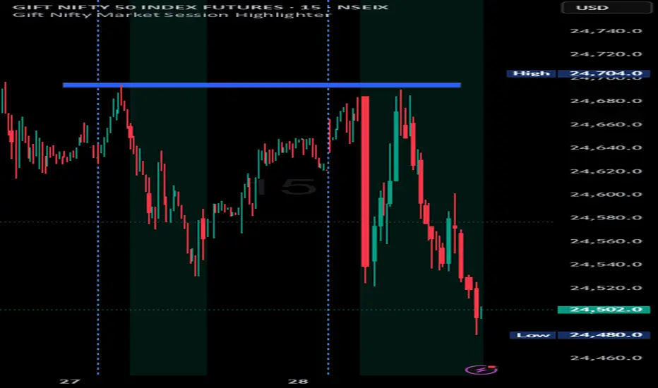
ORB Breakouts with alerts"ORB Breakouts with Alerts" is a utility indicator that highlights an Opening Range Breakout (ORB) setup during a user-defined intraday time window. It allows traders to visualize price consolidation ranges and receive alerts when price breaks above or below the session high/low.
🔧 Features:
*Customizable session time (start and end), adjustable to local time using a timezone offset.
*Automatically plots:
*A shaded box around the session's high and low.
*Horizontal lines at session high and low levels.
*Optional "BUY"/"SELL" labels to mark breakout directions.
*Visual breakout signals when price crosses above or below the session range.
*Built-in alerts to notify when breakouts occur.
*Configurable styling options including box color, highlight color, and label placement.
⚙️ How It Works:
*During the defined time range, the script tracks the highest high and lowest low.
*After the session ends:
*A box is drawn to represent the opening range.
*Breakouts above the high or below the low trigger visual markers and optional alerts.
*Alerts are limited to one per direction per day to reduce noise.
⚠️ This indicator is a technical analysis tool only and does not provide financial advice or trade recommendations. Always use with proper risk management and in conjunction with your trading plan.
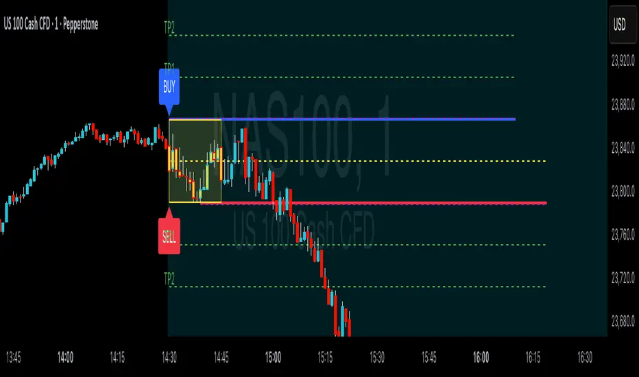
Key Session & LevelsThis indicator helps traders track key price levels for multiple timeframes and trading sessions. It plots:
Previous Day's High and Low (PD): Highlighting the high and low of the previous trading day.
Previous Week's High and Low (PW): Plotting the highest and lowest price levels for the past week.
Tokyo Session High and Low (Today): Displays the high and low levels for the Tokyo trading session (adjustable to your preferred time window).
London Session High and Low (Today): Tracks the high and low for the London trading session (also adjustable for your timezone and desired session window).
Features:
Customizable Time Zones: The indicator uses your preferred timezone to calculate session highs/lows.
Extendable Lines: Lines for each level extend to the right of the chart, providing continuous reference throughout the trading day.
Adjustable Settings: Fine-tune the visibility and width of the lines, and choose which levels to display (Previous Day, Previous Week, Tokyo, and London sessions).
Non-Repainting: This script uses historical data and only updates when new bars are confirmed, ensuring accurate and reliable signals.
Whether you're a day trader, swing trader, or just tracking key levels for strategic entries and exits, this tool provides quick visual reference to important price points across different trading sessions.
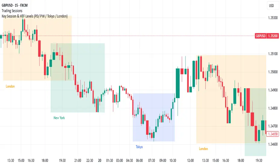
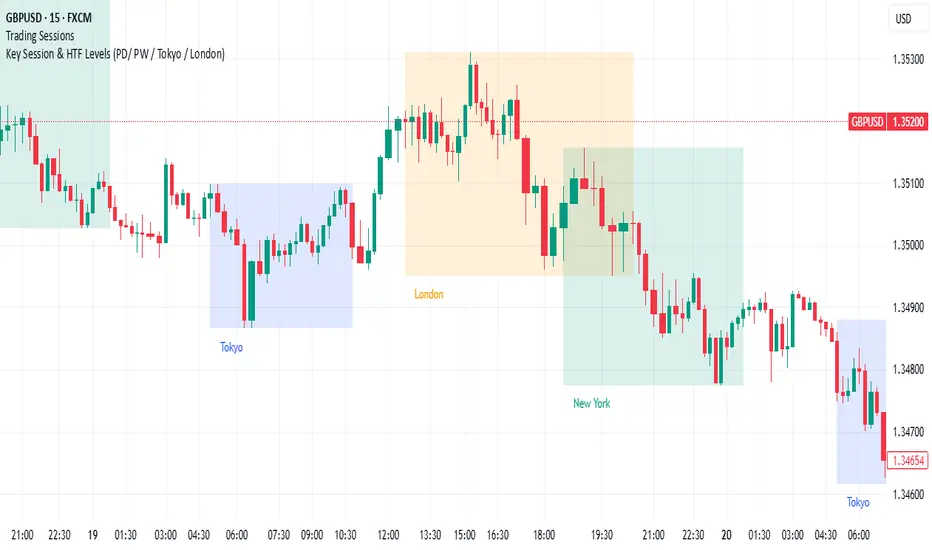
ORB & Sessions [Capitalize Labs]ORB & Sessions Indicator
The ORB & Sessions Indicator provides a structured way to analyze intraday price action by combining two well-established concepts: global trading sessions and Opening Range Breakouts (ORB). It is designed to help traders identify where liquidity forms, when volatility expands, and how price behaves around key session and range levels.
Market Sessions Framework
Displays New York, London, and Asian sessions directly on the chart.
Each session can be shown as a highlighted background zone, or with extended highs and lows for liquidity tracking.
Session highs and lows remain projected forward after the session ends, allowing traders to monitor sweeps, retests, and reactions throughout the day.
Session times are fully customizable and can be aligned with the trader’s own timezone or broker feed.
This structure helps traders place price action into context, whether during quiet Asian trading, London-driven volatility, or New York reversals.
Opening Range Breakouts (ORB)
Supports three independent ORBs, each with configurable session times.
During the defined ORB window, the indicator captures the high and low of the range and plots a live updating box.
Once the ORB closes, the range locks and projects breakout targets (T1 and T2) based on user-defined risk-to-reward multiples.
Alerts are included for breakouts of highs, lows, or target levels.
Traders can use a single ORB or multiple—for example, tracking an Asian ORB into London, or London into New York.
Visualization and Clarity
Color-coded boxes and levels for sessions and ORBs.
Labels such as “Range High” and “Range Low” ensure clarity without clutter.
Flexible display settings allow highlighting full zones, just lines, or minimal markers depending on preference.
Practical Applications
This indicator is useful for:
Liquidity and volatility analysis: Observe where session highs and lows form and how they influence later trading.
Breakout and reversal strategies: Use ORB ranges to define risk and plan target projections.
Time-based research: Explore how different session overlaps or ORBs affect markets like indices, FX, and commodities.
Risk planning: Built-in R-multiple targets provide a consistent framework for evaluating setups.
Why It’s Different
Instead of showing sessions and ORBs separately, this indicator integrates them into one framework. Traders can:
See when and where sessions open and establish range levels.
Define precise ORBs with customizable timing.
Track breakout levels and targets in real time with alerts.
The result is a clear, time-structured view of the trading day, helping traders align setups with session dynamics and opening range behavior.
This indicator does not generate buy or sell signals. It is an analytical and visualization tool, providing structure for traders to better interpret intraday price action.
